Note
Go to the end to download the full example code.
Typhoon Tracking and Axisymmetric Analysis#
This document demonstrates the process of tracking a typhoon’s center and performing axisymmetric analysis using mean sea level pressure (MSL), temperature, and precipitation data. The provided functions in easyclimate, implement the core algorithms for cyclone tracking and axisymmetric decomposition.
import numpy as np
import xarray as xr
import pandas as pd
import matplotlib.pyplot as plt
import cartopy.crs as ccrs
import easyclimate as ecl
loads meteorological reanalysis datasets (ERA5) for a typhoon. The datasets include:
Temperature (t_data): A multi-level atmospheric temperature field.
Mean Sea Level Pressure (slp_time, slp_data): MSL pressure data with time, latitude, and longitude dimensions. A single time slice (slp_data) is extracted for initial analysis.
Precipitation (tp_data): Total precipitation data, converted from its original units (
m/h) to millimeters per hour (mm/h) by multiplying by 1000 and updating the units attribute.
t_data = xr.open_dataset("test_t_typhoon_201919.nc").t

slp_time = xr.open_dataset("test_slp_typhoon_201919.nc").msl
slp_data = slp_time.isel(time = 0)

tp_data = xr.open_dataset("test_pr_typhoon_201919.nc").tp *1000
tp_data.attrs["units"] = "mm/h"
Tracking#
We uses the easyclimate.field.typhoon.track_cyclone_center_msl_only function to locate the typhoon center
at a single time step using MSL pressure data. The function takes the following inputs:
slp_data: A 2Dxarray.DataArraycontaining MSL pressure with latitude and longitude dimensions.sample_point: An initial guess for the cyclone center, like(longitude=140°, latitude=20°).
The function identifies local minima in the MSL pressure field using a 3x3 minimum filter (scipy.ndimage.minimum_filter)
with nearest boundary conditions to account for the grid edges. This ensures robust detection of low-pressure centers, which are characteristic of cyclones.
To be specific, the function computes the great-circle distance between the provided sample_point and all detected minima using the formula:
where \(\alpha\) is the central angle, and the closest minimum is selected as the cyclone center.
To refine the cyclone center beyond the grid resolution, the function applies biquadratic interpolation around the identified minimum. It constructs a quadratic function:
and solves for the extremum by setting the gradient to zero (i.e., \(\\nabla f = 0\)). The solution involves computing the inverse of the Hessian matrix:
to determine the offsets \(\Delta x\) and \(\Delta y\). If the determinant \(d = 0\), the grid-based minimum is used instead.
Here, we extends the tracking to multiple time steps by iterating over the time dimension of the slp_time dataset. For each time step:
The
easyclimate.field.typhoon.track_cyclone_center_msl_onlyfunction is called with the MSL data slice attime_item, the same initial guess(140, 20), and anindex_valueset to the current time index.Results are stored in a list (
track_list) and concatenated into a singlepandas.DataFrame(result) with columnslon,lat, andslp_min, indexed by time.
track_list = []

for time_item in np.arange(len(slp_time.time)):
    tmp = ecl.field.typhoon.track_cyclone_center_msl_only(slp_time.isel(time = time_item), (140, 20), index_value = [time_item])
    track_list.append(tmp)

result = pd.concat(track_list)
result
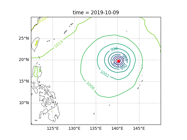
Here, we visualizes the MSL pressure field and the tracked typhoon center on a map.
fig, ax = ecl.plot.quick_draw_spatial_basemap(central_longitude=120)
ax.set_extent([120, 150, 5, 30], crs = ccrs.PlateCarree())


c = (slp_data/100).plot.contour(
    levels = 11,
    transform=ccrs.PlateCarree(),
    zorder = 1
)
ax.clabel(c)

ax.scatter(
    df_track["lon"][0], df_track['lat'][0],
    c="red",
    transform=ccrs.PlateCarree(),
    zorder = 2
)
<matplotlib.collections.PathCollection object at 0x7ff4209fbc10>
Axisymmetric Analysis#
Temperature (multi-level variable)#
This section performs axisymmetric analysis on the multi-level temperature data (t_data) using the easyclimate.field.typhoon.cyclone_axisymmetric_analysis function
The function transforms the data into a polar coordinate system centered on the typhoon (relocated to the North Pole) using spherical orthodrome transformation (Ritchie, 1987; Nakamura et al., 1997; Yamazaki, 2011). This involves:
Converting longitude-latitude coordinates to Cartesian coordinates:
\[x = \cos \lambda \sin \theta, \quad y = \sin \lambda \sin \theta, \quad z = \cos \theta\]Applying two rotations to align the cyclone center at the North Pole:
Rotate by \(-\theta_c\) around the y-axis.
Rotate by \(\lambda_c\) around the z-axis.
The combined rotation matrix is:
Interpolating the data onto a polar grid, e.g.,
polar_lon=np.arange(0, 360, 2)andpolar_lat=np.arange(80, 90.1, 1).
See also
https://www.dpac.dpri.kyoto-u.ac.jp/enomoto/pymetds/Typhoon.html
Ritchie, H. (1987). Semi-Lagrangian Advection on a Gaussian Grid. Monthly Weather Review, 115(2), 608-619. https://journals.ametsoc.org/view/journals/mwre/115/2/1520-0493_1987_115_0608_slaoag_2_0_co_2.xml
Nakamura, H., Nakamura, M., & Anderson, J. L. (1997). The Role of High- and Low-Frequency Dynamics in Blocking Formation. Monthly Weather Review, 125(9), 2074-2093. https://journals.ametsoc.org/view/journals/mwre/125/9/1520-0493_1997_125_2074_trohal_2.0.co_2.xml.
Yamazaki, A. (山崎 哲), 2011: The maintenance mechanism of atmospheric blocking. D.S. thesis, Kyushu University (Available online at http://hdl.handle.net/2324/21709, https://doi.org/10.15017/21709).
Finally, we decomposes the data into:
rotated: Interpolated data on the polar grid.rotated_symmetric: Azimuthal mean (axisymmetric component).rotated_asymmetric: Deviation from the azimuthal mean (asymmetric component).
temp_tc_polar_result = ecl.field.typhoon.cyclone_axisymmetric_analysis(
    t_data,
    (df_track["lon"][0], df_track['lat'][0])
)
temp_tc_polar_result
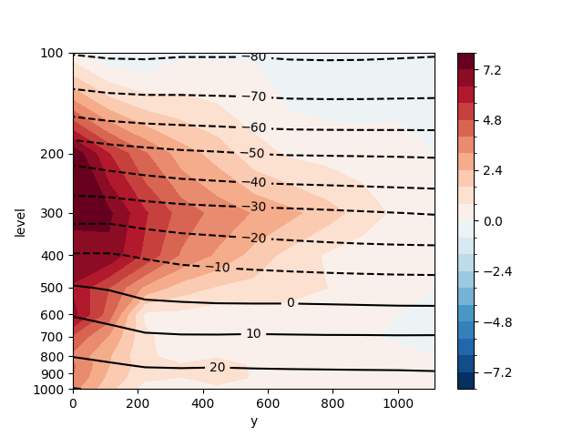
We processes the symmetric temperature component:
Anomaly Calculation:
r1computes the temperature anomaly by subtracting the value at the cyclone center (\(y=0\), corresponding to the North Pole in the transformed coordinates) from the symmetric component (ds_sym), highlighting radial variations in the warm core structure.Unit Conversion:
r2converts the symmetric temperature from Kelvin ( \(\mathrm{K}\) ) to Celsius ( \(\mathrm{^\circC}\) ) .
ds_sym = temp_tc_polar_result["rotated_symmetric"]
r1 = (ds_sym - ds_sym.isel(y = 0))
r2 = ecl.utility.transfer_data_temperature_units(ds_sym, "K", "degC")
Here, we visualizes the symmetric temperature anomaly and absolute temperature.
fig, ax = plt.subplots()
ecl.plot.set_p_format_axis()

r1.plot.contourf(
    ax = ax,
    levels = np.linspace(-8, 8, 21),
    yincrease = False
)

c = r2.plot.contour(
    levels= np.arange(-80, 80, 10),
    colors = "k",
    yincrease = False
)
ax.clabel(c)
<a list of 11 text.Text objects>
In this part, we extracts and prepares the asymmetric temperature component at the 850 hPa level for visualization:
ds_asym = temp_tc_polar_result["rotated_asymmetric"]
ds_asym850 = ds_asym.sel(level = 850)

ds_asym850_latlon = ds_asym850.swap_dims({'y': 'lat', 'polar_lon': 'lon'})
ds_asym850_latlon_0360 = ecl.plot.add_lon_cyclic(ds_asym850_latlon, inter = 2)
And visualizes the asymmetric temperature component at 850 hPa on a polar stereographic map.
fig, ax = plt.subplots(subplot_kw={"projection": ccrs.NorthPolarStereo()})

ecl.plot.draw_Circlemap_PolarStereo(
    ax=ax,
    lon_step=30,
    lat_step=2.5,
    lat_range=[80, 90],
    draw_labels=False,
    set_map_boundary_kwargs={"north_pad": 0.3, "south_pad": 0.4},
    gridlines_kwargs={"color": "grey", "alpha": 0.8, "linestyle": "--"},
)

(ds_asym850_latlon_0360 + 1e-13).plot.contourf(
    x = "lon", y = "lat",
    transform=ccrs.PlateCarree(),
    cmap = "RdBu_r",
    levels = 21
)
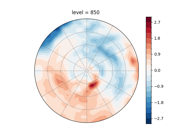
<cartopy.mpl.contour.GeoContourSet object at 0x7ff420f45a10>
Precipitation (single level variable)#
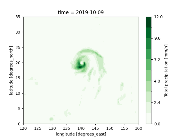
At first, we visualizes the precipitation field (tp_data) in its original longitude-latitude coordinates.
tp_data.plot.contourf(cmap = "Greens", levels = np.linspace(0, 12, 11))
<matplotlib.contour.QuadContourSet object at 0x7ff42171f910>
And then, we apply axisymmetric analysis to the single-level precipitation data.
pr_tc_polar_result = ecl.field.typhoon.cyclone_axisymmetric_analysis(
    tp_data,
    (df_track["lon"][0], df_track['lat'][0])
)
pr_tc_polar_result
Next, we prepare the rotated precipitation data for visualization.
pr_polardata = pr_tc_polar_result["rotated"].swap_dims({'y': 'lat', 'polar_lon': 'lon'})
pr_polardata = ecl.plot.add_lon_cyclic(pr_polardata, inter = 2)
And we visualizes the asymmetric precipitation component.
fig, ax = plt.subplots(subplot_kw={"projection": ccrs.NorthPolarStereo()})

ecl.plot.draw_Circlemap_PolarStereo(
    ax=ax,
    lon_step=30,
    lat_step=2.5,
    lat_range=[80, 90],
    draw_labels=False,
    set_map_boundary_kwargs={"north_pad": 0.3, "south_pad": 0.4},
    gridlines_kwargs={"color": "grey", "alpha": 0.4, "linestyle": "--"},
)

(pr_polardata + 1e-13).plot.contourf(
    x = "lon", y = "lat",
    transform=ccrs.PlateCarree(),
    cmap = "Greens",
    levels = np.linspace(0, 12, 11)
)
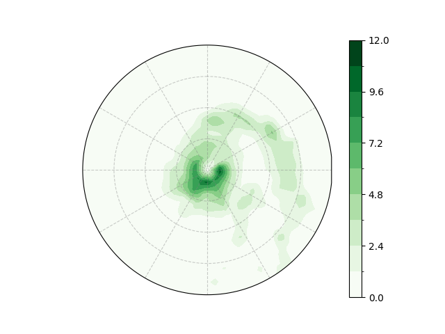
<cartopy.mpl.contour.GeoContourSet object at 0x7ff42170a490>
At this step, we will also perform coordinate dimension and data conversion.
ds_asym = pr_tc_polar_result["rotated_asymmetric"]

ds_asym_latlon = ds_asym.swap_dims({'y': 'lat', 'polar_lon': 'lon'})
ds_asym_latlon_0360 = ecl.plot.add_lon_cyclic(ds_asym_latlon, inter = 2)
At last, we visualize the asymmetric precipitation componen
fig, ax = plt.subplots(subplot_kw={"projection": ccrs.NorthPolarStereo()})

ecl.plot.draw_Circlemap_PolarStereo(
    ax=ax,
    lon_step=30,
    lat_step=2.5,
    lat_range=[80, 90],
    draw_labels=False,
    set_map_boundary_kwargs={"north_pad": 0.3, "south_pad": 0.4},
    gridlines_kwargs={"color": "grey", "alpha": 0.8, "linestyle": "--"},
)

(ds_asym_latlon_0360 + 1e-13).plot.contourf(
    x = "lon", y = "lat",
    transform=ccrs.PlateCarree(),
    cmap = "RdBu_r",
    levels = np.linspace(-4, 4, 21)
)
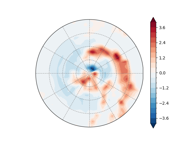
<cartopy.mpl.contour.GeoContourSet object at 0x7ff4215bc190>
Total running time of the script: (0 minutes 6.285 seconds)