Arctic Oscillation (AO) Index

Arctic Oscillation (AO) Index#

The Arctic Oscillation (AO) Index (or Monthly Northern Hemisphere Annular Mode (NAM) Index) is a key metric used to describe large-scale atmospheric variability in the Northern Hemisphere, particularly influencing mid-to-high latitude weather patterns. It is defined by the leading mode of Empirical Orthogonal Function (EOF) analysis of sea-level pressure (SLP) anomalies north of 20°N. The AO Index quantifies fluctuations in atmospheric pressure between the Arctic and mid-latitudes, with positive and negative phases reflecting distinct circulation patterns. In the positive phase, lower Arctic pressure and higher mid-latitude pressure strengthen westerly winds, confining cold air to polar regions, often leading to milder winters in North America and Europe. The negative phase, with higher Arctic pressure and weaker winds, allows cold air to move southward, causing colder, stormier weather in these regions.

The AO’s role in climate variability is significant, as it modulates temperature and precipitation, especially in winter. The AO Index, typically derived from monthly or seasonal SLP data, reflects the strength of the polar vortex, with positive values indicating a stronger vortex and negative values a weaker one. It is closely linked to the North Atlantic Oscillation (NAO) due to shared variability patterns.

The AO’s fluctuations are driven by internal atmospheric dynamics, stratospheric processes, and external forcings like sea surface temperatures. Its teleconnections make it a critical factor in seasonal weather predictions and long-term climate modeling. In a warming climate, Arctic amplification may alter AO dynamics, making its study essential for understanding future climate trends.

See also

  • Thompson, D. W. J., & Wallace, J. M. (1998). The Arctic oscillation signature in the wintertime geopotential height and temperature fields. Geophysical Research Letters, 25(9), 1297–1300. https://doi.org/10.1029/98gl00950

  • Fang, Z., Sun, X., Yang, X.-Q., & Zhu, Z. (2024). Interdecadal variations in the spatial pattern of the Arctic Oscillation Arctic center in wintertime. Geophysical Research Letters, 51, e2024GL111380. https://doi.org/10.1029/2024GL111380

  • Li, J., and J. X. L. Wang (2003), A modified zonal index and its physical sense, Geophys. Res. Lett., 30, 1632, doi: https://doi.org/10.1029/2003GL017441, 12.

  • Thompson, D. W. J. , & Wallace, J. M. . (1944). The Arctic oscillation signature in the wintertime geopotential height and temperature fields. Geophys. Res. Lett., doi: https://10.1029/98GL00950

Before proceeding with all the steps, first import some necessary libraries and packages

import easyclimate as ecl
import xarray as xr
import numpy as np
import matplotlib.pyplot as plt
import cartopy.crs as ccrs

Load monthly mean sea level pressure (SLP) data for the Northern Hemisphere The data is read from a NetCDF file containing SLP monthly means

slp_data = xr.open_dataset("slp_monmean_NH.nc").slp

Calculate seasonal mean for December-January-February (DJF) This aggregates the monthly data into winter seasonal means

<xarray.DataArray 'slp' (time: 78, lat: 29, lon: 144)> Size: 1MB
array([[[1010.59375, 1010.59375, 1010.59375, ..., 1010.59375,
         1010.59375, 1010.59375],
        [1010.3125 , 1010.34375, 1010.375  , ..., 1010.28125,
         1010.28125, 1010.3125 ],
        [1009.53125, 1009.46875, 1009.375  , ..., 1009.75   ,
         1009.6875 , 1009.59375],
        ...,
        [1018.     , 1017.875  , 1018.84375, ..., 1019.09375,
         1018.75   , 1018.28125],
        [1016.75   , 1016.75   , 1017.21875, ..., 1017.5625 ,
         1017.625  , 1017.1875 ],
        [1015.25   , 1015.375  , 1015.28125, ..., 1016.09375,
         1016.15625, 1015.71875]],

       [[1013.5208 , 1013.5208 , 1013.5208 , ..., 1013.5208 ,
         1013.5208 , 1013.5208 ],
        [1012.7083 , 1012.7292 , 1012.7708 , ..., 1012.6667 ,
         1012.6667 , 1012.6875 ],
        [1010.5208 , 1010.4167 , 1010.3125 , ..., 1010.8542 ,
         1010.75   , 1010.6042 ],
...
        [1018.9583 , 1018.8958 , 1020.0208 , ..., 1019.625  ,
         1019.5    , 1019.2083 ],
        [1017.5833 , 1017.9375 , 1018.7292 , ..., 1017.8125 ,
         1018.1667 , 1017.875  ],
        [1016.4167 , 1017.125  , 1017.5208 , ..., 1016.25   ,
         1016.6667 , 1016.5208 ]],

       [[1013.375  , 1013.375  , 1013.375  , ..., 1013.375  ,
         1013.375  , 1013.375  ],
        [1011.9375 , 1011.9792 , 1012.0208 , ..., 1011.8333 ,
         1011.8542 , 1011.9167 ],
        [1010.375  , 1010.3333 , 1010.2917 , ..., 1010.4375 ,
         1010.4167 , 1010.375  ],
        ...,
        [1018.7292 , 1018.3958 , 1019.25   , ..., 1019.8125 ,
         1019.5833 , 1019.1458 ],
        [1017.125  , 1017.0833 , 1017.4792 , ..., 1017.9792 ,
         1018.125  , 1017.5833 ],
        [1015.7292 , 1016.0417 , 1016.1875 , ..., 1016.125  ,
         1016.4375 , 1016.0833 ]]], shape=(78, 29, 144), dtype=float32)
Coordinates:
  * lat      (lat) float32 116B 90.0 87.5 85.0 82.5 80.0 ... 27.5 25.0 22.5 20.0
  * lon      (lon) float32 576B 0.0 2.5 5.0 7.5 10.0 ... 350.0 352.5 355.0 357.5
  * time     (time) datetime64[ns] 624B 1947-12-01 1948-12-01 ... 2024-12-01
Attributes:
    long_name:     Sea Level Pressure
    valid_range:   [ 870. 1150.]
    units:         millibars
    precision:     1
    var_desc:      Sea Level Pressure
    level_desc:    Sea Level
    statistic:     Mean
    parent_stat:   Other
    dataset:       NCEP Reanalysis Derived Products
    actual_range:  [ 955.56085 1082.5582 ]


Remove the seasonal cycle mean to obtain anomalies This creates anomalies by subtracting the long-term seasonal mean

<xarray.DataArray 'slp' (time: 78, lat: 29, lon: 144)> Size: 1MB
array([[[-2.9290771e+00, -2.9290771e+00, -2.9290771e+00, ...,
         -2.9290771e+00, -2.9290771e+00, -2.9290771e+00],
        [-2.1723022e+00, -2.1670532e+00, -2.1616821e+00, ...,
         -2.1343994e+00, -2.1570435e+00, -2.1476440e+00],
        [-1.6235962e+00, -1.5916748e+00, -1.5862427e+00, ...,
         -1.6635742e+00, -1.6454468e+00, -1.6486206e+00],
        ...,
        [ 9.3939209e-01,  9.8016357e-01,  1.1361084e+00, ...,
          7.1582031e-01,  7.6501465e-01,  8.2513428e-01],
        [ 7.7581787e-01,  7.9595947e-01,  9.1125488e-01, ...,
          5.8496094e-01,  6.4642334e-01,  7.5500488e-01],
        [ 4.8095703e-01,  4.1345215e-01,  3.1811523e-01, ...,
          5.7073975e-01,  6.0186768e-01,  5.6518555e-01]],

       [[-2.0141602e-03, -2.0141602e-03, -2.0141602e-03, ...,
         -2.0141602e-03, -2.0141602e-03, -2.0141602e-03],
        [ 2.2351074e-01,  2.1838379e-01,  2.3413086e-01, ...,
          2.5103760e-01,  2.2839355e-01,  2.2735596e-01],
        [-6.3403320e-01, -6.4373779e-01, -6.4874268e-01, ...,
         -5.5938721e-01, -5.8294678e-01, -6.3818359e-01],
...
          1.2470703e+00,  1.5150146e+00,  1.7521973e+00],
        [ 1.6091309e+00,  1.9834595e+00,  2.4216919e+00, ...,
          8.3496094e-01,  1.1881104e+00,  1.4425049e+00],
        [ 1.6476440e+00,  2.1634521e+00,  2.5576782e+00, ...,
          7.2698975e-01,  1.1123047e+00,  1.3672485e+00]],

       [[-1.4782715e-01, -1.4782715e-01, -1.4782715e-01, ...,
         -1.4782715e-01, -1.4782715e-01, -1.4782715e-01],
        [-5.4730225e-01, -5.3161621e-01, -5.1586914e-01, ...,
         -5.8233643e-01, -5.8410645e-01, -5.4345703e-01],
        [-7.7984619e-01, -7.2711182e-01, -6.6955566e-01, ...,
         -9.7607422e-01, -9.1625977e-01, -8.6737061e-01],
        ...,
        [ 1.6685791e+00,  1.5009766e+00,  1.5423584e+00, ...,
          1.4345703e+00,  1.5983276e+00,  1.6896973e+00],
        [ 1.1508179e+00,  1.1292725e+00,  1.1716919e+00, ...,
          1.0016479e+00,  1.1464233e+00,  1.1508179e+00],
        [ 9.6014404e-01,  1.0801392e+00,  1.2243652e+00, ...,
          6.0198975e-01,  8.8311768e-01,  9.2974854e-01]]],
      shape=(78, 29, 144), dtype=float32)
Coordinates:
  * lat      (lat) float32 116B 90.0 87.5 85.0 82.5 80.0 ... 27.5 25.0 22.5 20.0
  * lon      (lon) float32 576B 0.0 2.5 5.0 7.5 10.0 ... 350.0 352.5 355.0 357.5
  * time     (time) datetime64[ns] 624B 1947-12-01 1948-12-01 ... 2024-12-01
    month    (time) int64 624B 12 12 12 12 12 12 12 12 ... 12 12 12 12 12 12 12
Attributes:
    long_name:     Sea Level Pressure
    valid_range:   [ 870. 1150.]
    units:         millibars
    precision:     1
    var_desc:      Sea Level Pressure
    level_desc:    Sea Level
    statistic:     Mean
    parent_stat:   Other
    dataset:       NCEP Reanalysis Derived Products
    actual_range:  [ 955.56085 1082.5582 ]


Calculate Arctic Oscillation (AO) index using EOF method (Thompson & Wallace 1998) This performs EOF analysis on SLP anomalies north of 20°N to derive the AO index

<xarray.DataArray 'PC' (time: 78)> Size: 624B
array([-0.13789273, -1.36136224,  0.17735619,  0.88062118, -0.2129353 ,
        0.61538168, -0.14617055,  0.82448838,  1.40803593,  0.01084501,
        0.46198938,  0.20336214,  1.34985511,  0.09407199, -0.03657216,
        1.26591141,  0.06100193,  0.92674357,  1.47341691,  0.25968394,
        0.64145145,  2.39791578,  1.30622444,  0.42497478, -0.10463684,
       -1.2214392 ,  0.09991508, -0.93211804, -1.22233623,  2.0083876 ,
        0.56243371,  1.07133185,  0.20556959, -0.39572587,  0.19810533,
       -0.99517237, -0.37496718,  1.10574761,  1.04859641,  0.12535887,
        0.10322009, -2.66546857, -1.16177425, -0.662752  , -1.67955732,
       -2.06468711,  0.1944445 , -1.04616313,  0.59380495, -0.50431692,
        0.06580437, -0.79229132, -1.28876489,  0.77994097, -0.80616942,
        0.01642609,  0.19134825, -0.25406337,  0.62810255, -1.32004343,
       -1.01681461, -0.07190612,  2.71685131,  0.88742413, -0.59954162,
        0.86927108, -0.13355856, -1.16031679, -0.54596922, -1.17149519,
        0.1642507 , -0.39054768, -2.05494313,  1.3799055 , -0.95251467,
        0.23287031, -0.29608713, -0.25139045])
Coordinates:
  * time     (time) datetime64[ns] 624B 1947-12-01 1948-12-01 ... 2024-12-01
Attributes: (12/15)
    model:          EOF analysis
    software:       xeofs
    version:        3.0.4
    date:           2025-06-21 03:18:14
    n_modes:        2
    center:         False
    ...             ...
    sample_name:    sample
    feature_name:   feature
    random_state:   None
    compute:        True
    solver:         auto
    solver_kwargs:  {}


Calculate AO index using zonal mean SLP difference method (Li & Wang 2003) This computes the index as the normalized difference between 35°N and 65°N SLP

<xarray.DataArray 'slp' (time: 78)> Size: 312B
array([ 0.8052499 ,  4.3634815 , -1.2605035 , -1.710156  ,  1.578033  ,
       -1.2090005 , -0.54754215, -2.2022023 , -6.9559655 , -1.3279245 ,
       -0.99068666, -1.1872978 , -2.9158869 , -0.3270552 , -2.2568872 ,
       -6.8076696 , -0.19597752, -4.6988726 , -3.151997  , -0.8766823 ,
       -5.060997  , -9.11583   , -3.7444484 , -2.8222766 , -0.8740756 ,
        3.1170976 , -0.6909201 ,  2.2488987 ,  2.1816232 , -4.2153635 ,
       -2.1912057 , -1.6460643 , -1.8050665 , -1.5291634 , -0.57734895,
        3.215914  ,  0.3315078 , -3.9433742 , -1.9367197 ,  1.4089097 ,
        2.2672746 ,  8.049681  ,  5.3112535 ,  1.4390047 ,  4.7700214 ,
        5.5418687 ,  0.7047738 ,  2.9371235 , -3.1138027 ,  1.4530386 ,
        0.63142395,  3.588745  ,  4.384025  , -0.5550656 ,  3.6181107 ,
       -0.16198307, -0.07054477, -2.0740209 , -2.7117517 ,  6.165711  ,
        3.8844595 , -0.4756385 , -9.488225  , -4.8299484 ,  1.9110786 ,
       -1.359751  ,  2.1388004 ,  2.7669818 ,  4.5657372 ,  2.4385693 ,
        0.44942093,  1.6947916 ,  8.040273  , -0.79522365,  2.7276301 ,
        0.08425861,  1.8951628 ,  1.7004323 ], dtype=float32)
Coordinates:
  * time     (time) datetime64[ns] 624B 1947-12-01 1948-12-01 ... 2024-12-01
    month    (time) int64 624B 12 12 12 12 12 12 12 12 ... 12 12 12 12 12 12 12
Attributes:
    long_name:     Sea Level Pressure
    valid_range:   [ 870. 1150.]
    units:         millibars
    precision:     1
    var_desc:      Sea Level Pressure
    level_desc:    Sea Level
    statistic:     Mean
    parent_stat:   Other
    dataset:       NCEP Reanalysis Derived Products
    actual_range:  [ 955.56085 1082.5582 ]


Calculate correlation between the two AO index calculation methods Shows how well the two different methods agree in capturing AO variability

array([[ 1.        , -0.91460804],
       [-0.91460804,  1.        ]])

Apply Gaussian filter to smooth the AO index time series Uses a 9-month window to highlight lower-frequency variations

<xarray.DataArray (time: 78)> Size: 624B
array([-0.06684012, -0.03738386,  0.01740327,  0.0902167 ,  0.17215534,
        0.25441799,  0.32989301,  0.39384404,  0.44455718,  0.48298112,
        0.51213765,  0.53648328,  0.56049485,  0.58791096,  0.62065395,
        0.657719  ,  0.69528552,  0.72658512,  0.74295929,  0.73589188,
        0.69922804,  0.63170361,  0.53858446,  0.4312157 ,  0.32488131,
        0.2348372 ,  0.17173515,  0.13904575,  0.13214965,  0.14070868,
        0.15245402,  0.15722669,  0.14900611,  0.12585784,  0.08784106,
        0.03482265, -0.03490786, -0.12356304, -0.23133062, -0.35423373,
       -0.4826228 , -0.60257186, -0.69918375, -0.76041284, -0.78070406,
       -0.76195968, -0.71237885, -0.64386572, -0.56851125, -0.49566789,
       -0.43049288, -0.37428554, -0.32574092, -0.28226979, -0.24113723,
       -0.19974644, -0.15587431, -0.10784048, -0.05542158, -0.00119777,
        0.04903026,  0.08649593,  0.10179069,  0.08803279,  0.04338423,
       -0.02733525, -0.1138375 , -0.20257341, -0.28068094, -0.33844134,
       -0.37116568, -0.3795721 , -0.36828661, -0.34435419, -0.31530194,
       -0.28771077, -0.26673484, -0.25550605])
Coordinates:
  * time     (time) datetime64[ns] 624B 1947-12-01 1948-12-01 ... 2024-12-01


Perform linear regression between SLP anomalies and AO index Calculates the spatial pattern of SLP associated with AO variability

Add cyclic point for plotting (avoids gap at 0/360° longitude)

Prepare AO index data for plotting Converts time to year-only format for cleaner visualization

index_ao_bar = index_ao.copy(deep=True)
index_ao_bar['time'] = index_ao_bar['time'].dt.year.data

index_ao_filtered_bar = index_ao_filtered.copy(deep=True)
index_ao_filtered_bar['time'] = index_ao_filtered_bar['time'].dt.year.data

Create time series plot of AO index

fig, ax = plt.subplots(figsize = (10, 4))

# Plot bar chart of annual AO index values
ecl.plot.bar_plot_with_threshold(index_ao_bar, ax = ax)
# Overlay smoothed time series
index_ao_filtered_bar.plot(color = 'k', lw = 2, ax = ax)

ax.set_title("Arctic Oscillation (AO) Index")
Arctic Oscillation (AO) Index
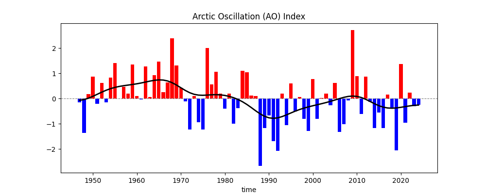
Text(0.5, 1.0, 'Arctic Oscillation (AO) Index')

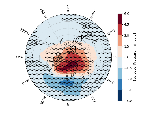
Create spatial map of SLP regression pattern associated with AO

fig, ax = plt.subplots(subplot_kw={"projection": ccrs.NorthPolarStereo()})

# Configure map appearance
ax.coastlines(edgecolor="black", linewidths=0.5)

# Add polar map elements (grid lines, labels)
ecl.plot.draw_Circlemap_PolarStereo(
    ax=ax,
    lon_step=30,
    lat_step=10,
    lat_range=[20, 90],
    draw_labels=True,
    set_map_boundary_kwargs={"north_pad": 0.3, "south_pad": 0.4},
    gridlines_kwargs={"color": "grey", "alpha": 0.5, "linestyle": "--"},
)

# Plot regression coefficients (SLP pattern)
slp_reg_ao_slope.plot.contourf(cmap="RdBu_r", levels=11, transform=ccrs.PlateCarree())
# Highlight statistically significant areas
ecl.plot.draw_significant_area_contourf(slp_reg_ao_pvalue, transform=ccrs.PlateCarree())
plot ao index

Total running time of the script: (0 minutes 3.510 seconds)