Note
Go to the end to download the full example code.
Oceanic Front#
The role of oceanic fronts in the midlatitude air–sea interaction remains unclear. Here, we defines new indexes to quantify the intensity and location of two basin-scale oceanic frontal zones in the wintertime North Pacific, i.e. the subtropical and subarctic frontal zones (STFZ, SAFZ). With these indexes, two typical modes, which are closely related to two large-scale sea surface temperature (SST) anomaly patterns resembling Pacific Decadal Oscillation (PDO) and North Pacific Gyre Oscillation (NPGO), respectively, are found in the oceanic front variabilities as well as in their associations with the midlatitude atmospheric eddy-driven jet. Corresponding to an PDO-like SST anomaly pattern, an enhanced STFZ occurs with a southward shifted SAFZ, which is associated with enhanced overlying atmospheric front, baroclinicity and transient eddy vorticity forcing, thus with an intensification of the westerly jet; and vice versa. On the other hand, corresponding to an NPGO-like SST pattern, an enhanced SAFZ occurs with a northward shifted STFZ, which is associated with a northward shift of the atmospheric front, baroclinicity, transient eddy vorticity forcing, and westerly jet; and vice versa. These results suggest that the basin-scale oceanic frontal zone is a key region for the midlatitude air–sea interaction in which the atmospheric transient eddy’s dynamical forcing is a key player in such an interaction.
See also
Wang, L., Yang, X.-Q., Yang, D., Xie, Q., Fang, J. and Sun, X. (2017), Two typical modes in the variabilities of wintertime North Pacific basin-scale oceanic fronts and associated atmospheric eddy-driven jet. Atmos. Sci. Lett, 18: 373-380. Website: https://doi.org/10.1002/asl.766
Wang, L., Hu, H. & Yang, X. The atmospheric responses to the intensity variability of subtropical front in the wintertime North Pacific. Clim Dyn 52, 5623–5639 (2019). https://doi.org/10.1007/s00382-018-4468-9
Huang, Q., Fang, J., Tao, L. et al. Wintertime ocean–atmosphere interaction processes associated with the SST variability in the North Pacific subarctic frontal zone. Clim Dyn 62, 1159–1177 (2024). https://doi.org/10.1007/s00382-023-06958-6
Fang, Z., Sun, X., Yang, X.-Q., & Zhu, Z. (2024). Interdecadal variations in the spatial pattern of the Arctic Oscillation Arctic center in wintertime. Geophysical Research Letters, 51, e2024GL111380. https://doi.org/10.1029/2024GL111380
姚瑶. (2018). 北太平洋风暴轴与中纬度海洋锋的相互作用研究(博士学位论文,国防科技大学). 博士 https://link.cnki.net/doi/10.27052/d.cnki.gzjgu.2018.000410.
Before proceeding with all the steps, first import some necessary libraries and packages
import numpy as np
import easyclimate as ecl
import cartopy.crs as ccrs
import cartopy.feature as cfeature
import matplotlib.pyplot as plt
import matplotlib.patches as patches
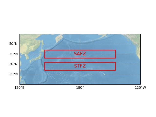
We sets up a cartographic projection (Plate Carrée) and creates a base map to visualize the study area. It restricts the spatial extent to the North Pacific (120°E–240°E, 10°N–60°N) and overlays grid lines with labeled coordinates. Rectangular patches are added to demarcate the Subtropical Frontal Zone (STFZ, 145°E–215°E, 24°N–32°N) and Subarctic Frontal Zone (SAFZ, 145°E–215°E, 36°N–44°N), with text labels for clarity. This establishes the geographical context for subsequent frontal zone analyses.
proj_trans = ccrs.PlateCarree()
fig, ax = plt.subplots(subplot_kw={'projection': ccrs.PlateCarree(central_longitude = 110)})

ax.stock_img()
ax.set_extent([120, 240, 10, 60], crs = proj_trans)

# Grid line
gl = ax.gridlines(draw_labels=True, color="grey",alpha = 0.5, linestyle="--")
gl.top_labels = False
gl.right_labels = False
gl.left_labels = True
gl.bottom_labels = True

# STFZ
rect1 = patches.Rectangle((145, 24), 70, 8, ec = "r", fc = "none", lw = 2, transform = proj_trans)
ax.add_patch(rect1)
ax.text(180 + 0, 28 + 0,'STFZ', size = 14, c = 'r', transform = proj_trans, horizontalalignment='center', verticalalignment='center')

# SAFZ
rect2 = patches.Rectangle((145, 36), 70, 8, ec = "r", fc = "none", lw = 2, transform = proj_trans)
ax.add_patch(rect2)
ax.text(180 + 0, 40 + 0,'SAFZ', size = 14, c = 'r', transform = proj_trans, horizontalalignment='center', verticalalignment='center')
Text(180, 40, 'SAFZ')
Here, we import the Optimum Interpolation Sea Surface Temperature (OISST) tutorial dataset using easyclimate, extracting the sst variable. The dataset is printed to display its structure (dimensions, coordinates, and metadata), ensuring the input data is correctly loaded for further processing.
sst_data = ecl.open_tutorial_dataset('sst_mnmean_oisst').sst
sst_data
This block calculates the winter (December–January–February, DJF) seasonal mean SST from the monthly data using easyclimate.calc_seasonal_mean.
It then derives the long-term (time-mean) winter SST climatology over the extended North Pacific (110°E–250°E, 0°N–80°N).
Additionally, the meridional gradient of SST (\(\mathrm{d}SST/\mathrm{d}y\)) is computed using easyclimate.calc_lat_gradient
(with a sign inversion to align with standard gradient conventions) and averaged over time to obtain its climatological mean.
These variables are critical for quantifying oceanic frontal intensity (via \(\mathrm{d}SST/\mathrm{d}y\)) and spatial patterns.
sst_data_DJF_mean = ecl.calc_seasonal_mean(sst_data, extract_season="DJF")
sst_data_DJF_longmean = sst_data_DJF_mean.mean(dim = "time").sel(lon = slice(110, 250), lat = slice(0, 80))

dtdy_data_DJF_mean = ecl.calc_lat_gradient(sst_data_DJF_mean).sel(lon = slice(110, 250), lat = slice(0, 80)) *(-1)
dtdy_data_DJF_longmean = dtdy_data_DJF_mean.mean(dim = "time")
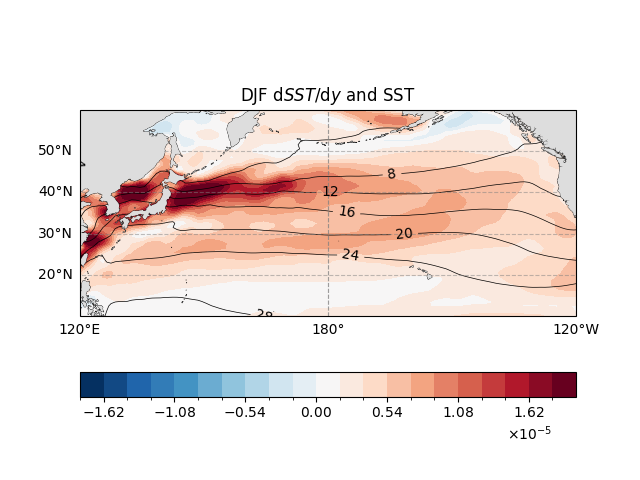
Next, The blocks visualize the long-term winter SST and its meridional gradient. Using a Plate Carrée projection centered at 180°E,
it overlays black SST contours (4–30℃, 4℃ intervals) to show surface temperature structure.
The \(\mathrm{d}SST/\mathrm{d}y\) field is plotted as a filled contour (range: \(-1.8 \times 10^{-5} \sim 1.8 \times 10^{-5}\) ℃/m) to
highlight regions of strong oceanic fronts (positive \(\mathrm{d}SST/\mathrm{d}y\) indicates northward SST increase).
Land areas are shaded to emphasize marine features. A horizontal colorbar is added for \(\mathrm{d}SST/\mathrm{d}y\),
with scientific notation formatting. This figure contextualizes frontal zones within the broader SST climatology.
proj_trans = ccrs.PlateCarree()
fig, ax = ecl.plot.quick_draw_spatial_basemap(central_longitude=180)

ax.set_extent([120, 240, 10, 60], crs = proj_trans)
ax.add_feature(cfeature.LAND, facecolor = '#DDDDDD', zorder = 2)

# SST
fig1 = sst_data_DJF_longmean.plot.contour(
    colors="k",
    linewidths = 0.5,
    levels=np.arange(4, 30, 4),
    transform = ccrs.PlateCarree(),
    zorder = 1,
)
ax.clabel(fig1, inline = True, fontsize = 10, colors = "k")

# dSST/dy
fig2 = dtdy_data_DJF_longmean.plot.contourf(
    levels=np.linspace(-1.8*1e-5, 1.8*1e-5, 21),
    transform = ccrs.PlateCarree(),
    add_colorbar=False,
    zorder = 0,
)
cb1 = fig.colorbar(fig2, ax = ax, orientation = 'horizontal', pad = 0.15, extendrect = True)
cb1.set_label('')
cb1.formatter.set_powerlimits((0, 0))
cb1.formatter.set_useMathText(True)

ax.set_title("DJF ${\\mathrm{d}SST}/{\\mathrm{d}y}$ and SST")
Text(0.5, 1.0, 'DJF ${\\mathrm{d}SST}/{\\mathrm{d}y}$ and SST')
This section uses easyclimate utility functions to quantify frontal zone variability:
easyclimate.field.ocean.oceanic_front.calc_intensity_STFZ: Computes the area-averaged \(\mathrm{d}SST/\mathrm{d}y\) within predefined STFZ regions to represent frontal intensity.easyclimate.field.ocean.oceanic_front.calc_intensity_SAFZ: Computes the area-averaged \(\mathrm{d}SST/\mathrm{d}y\) within predefined SAFZ regions to represent frontal intensity.easyclimate.field.ocean.oceanic_front.calc_location_STFZ: Determines the latitude of maximum \(\mathrm{d}SST/\mathrm{d}y\) within each zone to track STFZ position.easyclimate.field.ocean.oceanic_front.calc_location_SAFZ: Determines the latitude of maximum \(\mathrm{d}SST/\mathrm{d}y\) within each zone to track SAFZ position.easyclimate.field.ocean.oceanic_front.calc_location_line_STFZ: Generates longitude-dependent positional lines (latitude vs. longitude) for STFZ, capturing their zonal structure.easyclimate.field.ocean.oceanic_front.calc_location_SAFZ: Generates longitude-dependent positional lines (latitude vs. longitude) for SAFZ, capturing their zonal structure.
Long-term means of these positional lines are computed to establish climatological frontal boundaries.
intensity_STFZ_DJF = ecl.field.ocean.calc_intensity_STFZ(dtdy_data_DJF_mean)
intensity_SAFZ_DJF = ecl.field.ocean.calc_intensity_SAFZ(dtdy_data_DJF_mean)
location_STFZ_DJF = ecl.field.ocean.calc_location_STFZ(dtdy_data_DJF_mean)
location_SAFZ_DJF = ecl.field.ocean.calc_location_SAFZ(dtdy_data_DJF_mean)

line_STFZ_DJF = ecl.field.ocean.calc_location_line_STFZ(dtdy_data_DJF_mean)
line_SAFZ_DJF = ecl.field.ocean.calc_location_line_SAFZ(dtdy_data_DJF_mean)
line_STFZ_DJF_longmean = line_STFZ_DJF.mean(dim = "time")
line_SAFZ_DJF_longmean = line_SAFZ_DJF.mean(dim = "time")
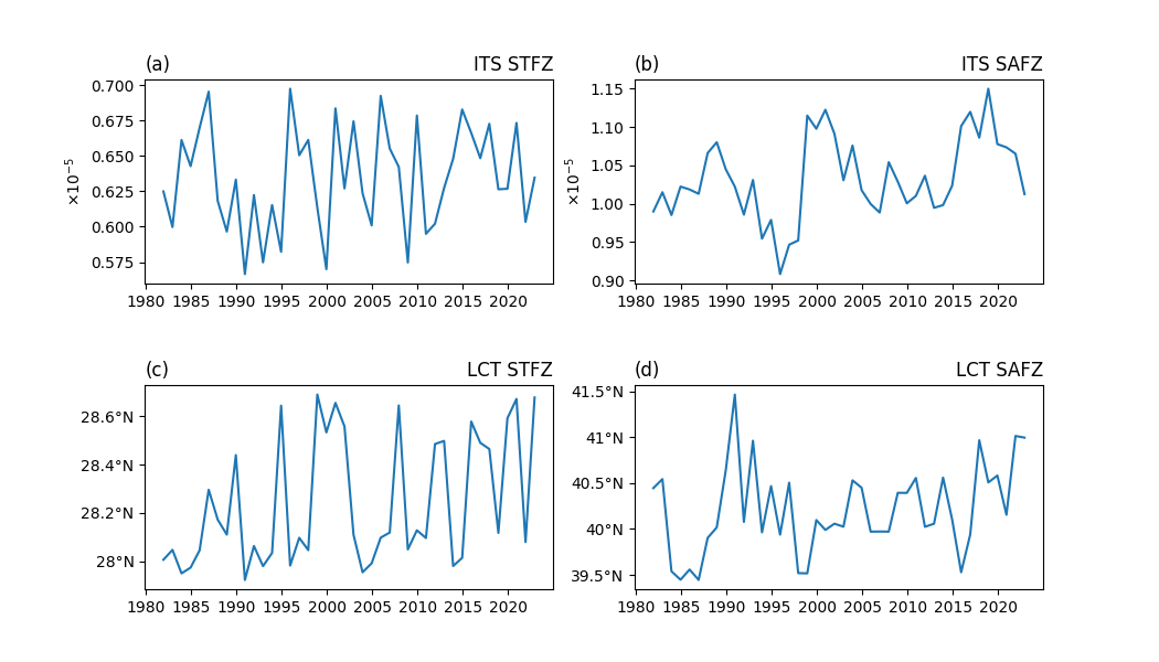
This code creates a 2×2 subplot grid to visualize frontal zone dynamics:
Top row: Time series of STFZ and SAFZ intensity (multiplied by \(10^5\) for readability), with y-labels indicating units (\(- 10^{-5}\) ℃/m).
Bottom row: Time series of STFZ and SAFZ meridional location (latitude, °N), with latitude-formatted axes.
Subplots are labeled (a)–(d) for reference, and x-axis labels are removed for consistency. This figure highlights interannual variations in frontal strength and position, key for identifying modes of variability (e.g., PDO/NPGO associations).
titleleft_fontsize = 22
titleright_fontsize = 20
titleleft_pad = 10
decimal_places = 2

fig, ax = plt.subplots(2, 2, figsize = (10.5, 6))
fig.subplots_adjust(hspace = 0.5)

# --------------------------------------------------
# STFZ Intensity
axi = ax[0, 0]

(intensity_STFZ_DJF *1e5).plot(ax = axi)

axi.set_ylabel('$\\times 10^{-5}$')

axi.set_title("ITS STFZ", loc = 'right')
axi.set_title("")
axi.set_title("(a)", loc = 'left')

# --------------------------------------------------
# SAFZ Intensity
axi = ax[0, 1]

(intensity_SAFZ_DJF *1e5).plot(ax = axi)
axi.set_ylabel('$\\times 10^{-5}$')

axi.set_title("ITS SAFZ", loc = 'right')
axi.set_title("")
axi.set_title("(b)", loc = 'left')

# --------------------------------------------------
# STFZ Location
axi = ax[1, 0]

(location_STFZ_DJF *1).plot(ax = axi)

axi.set_title("LCT STFZ", loc = 'right')
axi.set_title("")
axi.set_title("(c)", loc = 'left')

# --------------------------------------------------
# SAFZ Location
axi = ax[1, 1]

line1, = (location_SAFZ_DJF *1).plot(ax = axi)

axi.set_title("LCT SAFZ", loc = 'right')
axi.set_title("")
axi.set_title("(d)", loc = 'left')


for axi in ax.flat:
    axi.set_xlabel('')

for axi in [ax[1, 0], ax[1, 1]]:
    ecl.plot.set_lat_format_axis(ax = axi)
Finally, we revisits the spatial plot of winter \(\mathrm{d}SST/\mathrm{d}y\) but adds the long-term mean positional lines of STFZ and SAFZ (black lines).
These lines, derived from the zonal average of line_STFZ_DJF_longmean and line_SAFZ_DJF_longmean,
visually validate the frontal zone definitions by aligning with peak \(\mathrm{d}SST/\mathrm{d}y\) regions.
The figure confirms that the positional lines coincide with the core of the oceanic fronts,
ensuring the indices accurately represent frontal structure.
proj_trans = ccrs.PlateCarree()
fig, ax = ecl.plot.quick_draw_spatial_basemap(central_longitude=180)

ax.set_extent([120, 240, 10, 60], crs = proj_trans)
ax.add_feature(cfeature.LAND, facecolor = '#DDDDDD', zorder = 2)

# Line
line_STFZ_DJF_longmean.plot(ax = ax, color = 'black', zorder = 3, transform = proj_trans)
line_SAFZ_DJF_longmean.plot(ax = ax, color = 'black', zorder = 3, transform = proj_trans)

# dSST/dy
fig2 = dtdy_data_DJF_longmean.plot.contourf(
    levels=np.linspace(-1.8*1e-5, 1.8*1e-5, 21),
    transform = ccrs.PlateCarree(),
    add_colorbar=False,
    zorder = 0,
)
cb1 = fig.colorbar(fig2, ax = ax, orientation = 'horizontal', pad = 0.15, extendrect = True)
cb1.set_label('')
cb1.formatter.set_powerlimits((0, 0))
cb1.formatter.set_useMathText(True)

ax.set_title("DJF ${\\mathrm{d}SST}/{\\mathrm{d}y}$ and Line")

Text(0.5, 1.0, 'DJF ${\\mathrm{d}SST}/{\\mathrm{d}y}$ and Line')
Total running time of the script: (0 minutes 7.517 seconds)