Note
Go to the end to download the full example code.
KF Filter and Hovmöller Diagram#
The KF filter is a specialized spectral analysis technique designed to isolate and study tropical atmospheric waves by decomposing meteorological fields into their wavenumber-frequency components. Unlike traditional Fourier methods, the W-K filter applies a symmetric/antisymmetric separation to distinguish between different wave types, such as Kelvin waves, Rossby waves, and mixed Rossby-gravity waves, based on their theoretical dispersion relations. This approach is particularly effective in identifying convectively coupled waves, where tropical rainfall and large-scale circulation interact. In meteorology, the W-K filter is widely used to analyze Madden-Julian Oscillation (MJO) dynamics, monsoon variability, and other tropical wave disturbances, providing insights into their propagation characteristics and impacts on weather systems.
See also
Wheeler, M., & Kiladis, G. N. (1999). Convectively Coupled Equatorial Waves: Analysis of Clouds and Temperature in the Wavenumber–Frequency Domain. Journal of the Atmospheric Sciences, 56(3), 374-399. https://journals.ametsoc.org/view/journals/atsc/56/3/1520-0469_1999_056_0374_ccewao_2.0.co_2.xml
Kiladis, G. N., Thorncroft, C. D., & Hall, N. M. J. (2006). Three-Dimensional Structure and Dynamics of African Easterly Waves. Part I: Observations. Journal of the Atmospheric Sciences, 63(9), 2212-2230. https://doi.org/10.1175/JAS3741.1
Hall, N. M. J., Kiladis, G. N., & Thorncroft, C. D. (2006). Three-Dimensional Structure and Dynamics of African Easterly Waves. Part II: Dynamical Modes. Journal of the Atmospheric Sciences, 63(9), 2231-2245. https://doi.org/10.1175/JAS3742.1
Thorncroft, C. D., Hall, N. M. J., & Kiladis, G. N. (2008). Three-Dimensional Structure and Dynamics of African Easterly Waves. Part III: Genesis. Journal of the Atmospheric Sciences, 65(11), 3596-3607. https://doi.org/10.1175/2008JAS2575.1
Before proceeding with all the steps, first import some necessary libraries and packages
import numpy as np
import xarray as xr
import matplotlib.pyplot as plt
import cartopy.crs as ccrs
import easyclimate as ecl
Preprocessed data
Tip
You can download following datasets here:
lats, latn = -20, 20

olr_data = xr.open_dataset('olr-daily_v01r02_19800101_20231231.nc', chunks='auto').sel(lat=slice(lats,latn)).olr
olr_daily_smoothed = ecl.variability.remove_smooth_daily_annual_cycle_mean(
    olr_data, extract_time_range = slice('2017-01-01','2018-12-31')
)

# target grid
target_grid = xr.Dataset()
target_grid['lat'] = olr_daily_smoothed.lat.data
target_grid['lon'] = olr_daily_smoothed.lon.thin(lon = 5).data

olr_data_interpolated = ecl.interp.interp_mesh2mesh(olr_daily_smoothed, target_grid = target_grid)
olr_data_interpolated = ecl.utility.get_compress_xarraydata(olr_data_interpolated)
olr_data_interpolated.to_netcdf("olr_smooth_data.nc")
The example here is to avoid longer calculations, thus we open the pre-processed result data directly.
olr_data_interpolated = xr.open_dataset("olr_smooth_data.nc").olr
olr_data_interpolated
Filtering equatorial waves with kf_filter
lf_result = ecl.filter.kf_filter_lf_wave(olr_data_interpolated, steps_per_day = 1)
mjo_result = ecl.filter.kf_filter_mjo_wave(olr_data_interpolated, steps_per_day = 1)
er_result = ecl.filter.kf_filter_er_wave(olr_data_interpolated, steps_per_day = 1)
kelvin_result = ecl.filter.kf_filter_kelvin_wave(olr_data_interpolated, steps_per_day = 1)
mt_result = ecl.filter.kf_filter_mt_wave(olr_data_interpolated, steps_per_day = 1)
mrg_result = ecl.filter.kf_filter_mrg_wave(olr_data_interpolated, steps_per_day = 1)
td_result = ecl.filter.kf_filter_td_wave(olr_data_interpolated, steps_per_day = 1)
lf_result
/home/runner/work/easyclimate/easyclimate/src/easyclimate/filter/kf_filter.py:212: RuntimeWarning: invalid value encountered in sqrt
  freq = (beta * c) ** 0.5
/home/runner/work/easyclimate/easyclimate/src/easyclimate/filter/kf_filter.py:215: RuntimeWarning: invalid value encountered in sqrt
  freq = k * c * (0.5 + 0.5 * (1 + 4 * beta / (k**2 * c)) ** 0.5)
/home/runner/work/easyclimate/easyclimate/src/easyclimate/filter/kf_filter.py:217: RuntimeWarning: invalid value encountered in sqrt
  freq = k * c * (0.5 - 0.5 * (1 + 4 * beta / (k**2 * c)) ** 0.5)
Extract data in a specified time range
time1, time2 = '2017-12-01', '2018-02-28'
lon1, lon2, lats, latn = 39, 181, 5, 15

mjo_result_ave = mjo_result.sel(time=slice(time1,time2),lat=slice(lats,latn),lon=slice(lon1,lon2)).mean(dim = 'lat')
mrg_result_ave = mrg_result.sel(time=slice(time1,time2),lat=slice(lats,latn),lon=slice(lon1,lon2)).mean(dim = 'lat')
td_result_ave = td_result.sel(time=slice(time1,time2),lat=slice(lats,latn),lon=slice(lon1,lon2)).mean(dim = 'lat')
lf_result_ave = lf_result.sel(time=slice(time1,time2),lat=slice(lats,latn),lon=slice(lon1,lon2)).mean(dim = 'lat')
lf_result_ave
The Hovmöller Diagram is a powerful visualization tool that plots atmospheric or oceanic variables along one spatial axis (e.g., longitude or latitude) against time, revealing propagating wave patterns and persistent anomalies. By compressing spatiotemporal data into a single image, it allows meteorologists to track the phase speed, direction, and life cycle of large-scale waves, such as equatorial Kelvin waves or extratropical Rossby wave trains. In tropical meteorology, Hovmöller diagrams are frequently used to study the eastward progression of the MJO or the westward movement of tropical cyclones, while in climate science, they help diagnose teleconnections like the El Niño-Southern Oscillation (ENSO) influence on global weather. This method is essential for validating model simulations and understanding the organization of atmospheric disturbances over time.
See also
Persson, Anders. “The Story of the Hovmöller Diagram: An (Almost) Eyewitness Account”. Bulletin of the American Meteorological Society 98.5 (2017): 949-957. https://doi.org/10.1175/BAMS-D-15-00234.1 Web.
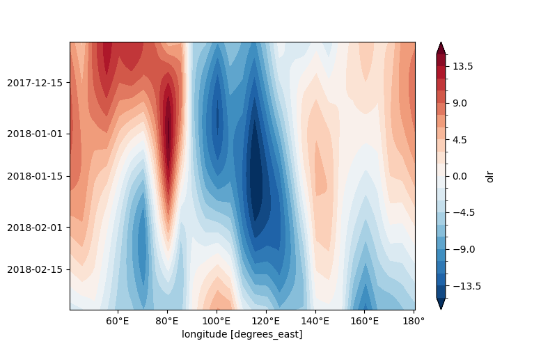
The first is given for equatorial waves with a frequency greater than 120 days of slow variation
fig, ax = plt.subplots(figsize = (8, 5))

lf_result_ave.plot.contourf(
    yincrease = False,
    levels = np.linspace(-15, 15, 21),
    cbar_kwargs={"location": "right", "aspect": 30},
)
ecl.plot.set_lon_format_axis()
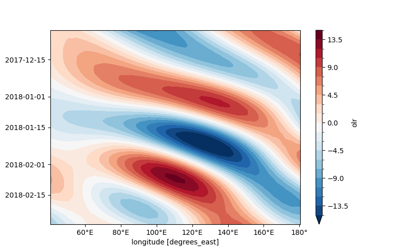
The MJO wave is extracted here.
The Madden–Julian Oscillation (MJO) is the major fluctuation in tropical weather on weekly to monthly timescales. It can be characterised as an eastward moving pulse or wave of cloud and rainfall near the equator that typically recurs every 30 to 60 days.
fig, ax = plt.subplots(figsize = (8, 5))

mjo_result_ave.plot.contourf(
    yincrease = False,
    levels = np.linspace(-15, 15, 21),
    cbar_kwargs={"location": "right", "aspect": 30},
)
ecl.plot.set_lon_format_axis()
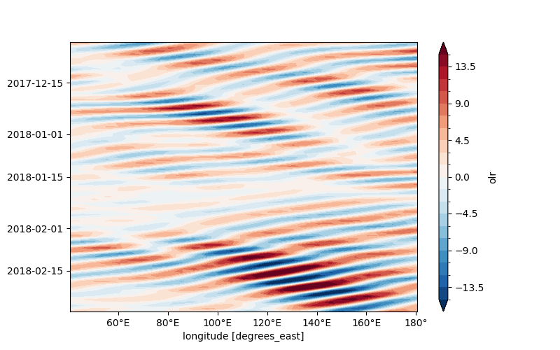
The mixed Rossby-Gravity (MRG) waves are extracted here.
The MRG waves move towards the west, but MRG waves have their pressure centres arranged anti-symmetrically on either side of the equator. This means a low pressure centre on one side of the equator will be opposite a high pressure centre in the other hemisphere. Satellite analysis of mixed Rossby-Gravity waves shows favoured zones for deep convection, often with thunderstorm clusters, in an antisymmetric arrangement about the equator. Their speed of movement to the west is faster than that of an ER wave.
fig, ax = plt.subplots(figsize = (8, 5))

mrg_result_ave.plot.contourf(
    yincrease = False,
    levels = np.linspace(-15, 15, 21),
    cbar_kwargs={"location": "right", "aspect": 30},
)
ecl.plot.set_lon_format_axis()
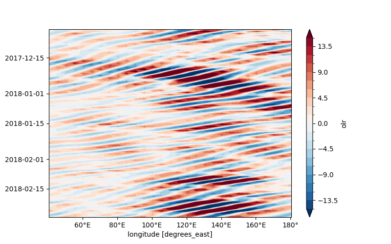
The tropical depression (TD) waves are extracted here
fig, ax = plt.subplots(figsize = (8, 5))

td_result_ave.plot.contourf(
    yincrease = False,
    levels = np.linspace(-15, 15, 21),
    cbar_kwargs={"location": "right", "aspect": 30},
)
ecl.plot.set_lon_format_axis()
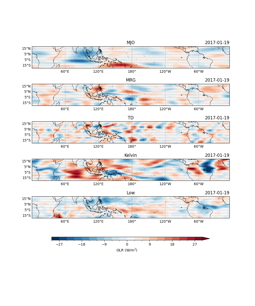
Finally we give the spatial planes of various equatorial waves
fig, ax = plt.subplots(
    nrows=5,
    figsize = (10, 12),
    subplot_kw={
        "projection": ccrs.PlateCarree(central_longitude=180)
    },
)
for axi in ax.flat:
    axi.gridlines(draw_labels=["bottom", "left"], color = "grey", alpha = 0.5, linestyle = "--")
    axi.coastlines(edgecolor='k', linewidths=0.5)

def get_date_str(data):
    return str(data['time'].data)[:10]

axi = ax[0]
data = mjo_result.isel(time = 18)
data.sel(lat = slice(-20, 20)).plot.contourf(
    ax = axi,
    levels = np.linspace(-30, 30, 21),
    transform = ccrs.PlateCarree(),
    add_colorbar = False,
)
axi.set_title("MJO")
axi.set_title(get_date_str(data), loc = 'right')

axi = ax[1]
data = mrg_result.isel(time = 18)
data.sel(lat = slice(-20, 20)).plot.contourf(
    ax = axi,
    levels = np.linspace(-30, 30, 21),
    transform = ccrs.PlateCarree(),
    add_colorbar = False,
)
axi.set_title("MRG")
axi.set_title(get_date_str(data), loc = 'right')

axi = ax[2]
data = td_result.isel(time = 18)
data.sel(lat = slice(-20, 20)).plot.contourf(
    ax = axi,
    levels = np.linspace(-30, 30, 21),
    transform = ccrs.PlateCarree(),
    add_colorbar = False,
)
axi.set_title("TD")
axi.set_title(get_date_str(data), loc = 'right')

axi = ax[3]
data = kelvin_result.isel(time = 18)
data.sel(lat = slice(-20, 20)).plot.contourf(
    ax = axi,
    levels = np.linspace(-30, 30, 21),
    transform = ccrs.PlateCarree(),
    add_colorbar = False,
)
axi.set_title("Kelvin")
axi.set_title(get_date_str(data), loc = 'right')

axi = ax[4]
data = lf_result.isel(time = 18)
bar_sample = data.sel(lat = slice(-20, 20)).plot.contourf(
    ax = axi,
    levels = np.linspace(-30, 30, 21),
    transform = ccrs.PlateCarree(),
    add_colorbar = False,
)
axi.set_title("Low")
axi.set_title(get_date_str(data), loc = 'right')

axi_item = ax.flatten()
cb1 = fig.colorbar(bar_sample, ax = axi_item, orientation = 'horizontal', pad = 0.08, aspect = 50, shrink = 0.8, extendrect = False)
cb1.set_label('OLR (W/$\\mathrm{m^2}$)')
Total running time of the script: (0 minutes 9.594 seconds)