Wheeler-Kiladis Space-Time Spectra

The Wheeler-Kiladis (WK) Space-Time Spectra is a diagnostic tool used in meteorology to analyze tropical atmospheric waves by decomposing their variability in both wavenumber (space) and frequency (time) domains. It extends traditional Fourier analysis by applying a two-dimensional (2D) spectral decomposition to isolate and characterize different wave modes (e.g., Kelvin waves, Rossby waves, and mixed Rossby-gravity waves) based on their dispersion relations.

Key Features

• Uses symmetrical (eastward/westward) and antisymmetrical (north-south) Fourier transforms to separate wave types.

• Compares observed spectra with theoretical dispersion curves of shallow-water waves to identify dominant modes.

• Helps distinguish convectively coupled waves (linked to tropical rainfall) from uncoupled waves.

Applications in Meteorology

1. Tropical Wave Analysis: Identifies and tracks Kelvin waves, equatorial Rossby waves, and Madden-Julian Oscillation (MJO) signals.

2. Convective Coupling Studies: Examines how waves interact with tropical convection (e.g., in monsoon systems).

3. Model Validation: Evaluates whether climate models correctly simulate tropical wave dynamics.

4. Extreme Weather Prediction: Helps understand precursors to tropical cyclogenesis and organized convection.

The WK method is particularly useful for studying large-scale tropical variability and remains a fundamental tool in tropical meteorology and climate research.

Before proceeding with all the steps, first import some necessary libraries and packages

import xarray as xr
import matplotlib.pyplot as plt
import easyclimate as ecl

The example here is to avoid longer calculations, thus we open the pre-processed result data directly.

Tip

You can download following datasets here: Download olr_smooth_data.nc

data = xr.open_dataset('olr_smooth_data.nc')['olr'].sel(lat = slice(-15, 15))
data

<xarray.DataArray 'olr' (time: 730, lat: 30, lon: 72)> Size: 6MB
[1576800 values with dtype=float32]
Coordinates:
  * time       (time) datetime64[ns] 6kB 2017-01-01T12:00:00 ... 2018-12-31T1...
    dayofyear  (time) int64 6kB ...
  * lon        (lon) float32 288B 0.5 5.5 10.5 15.5 ... 340.5 345.5 350.5 355.5
  * lat        (lat) float32 120B -14.5 -13.5 -12.5 -11.5 ... 12.5 13.5 14.5
Attributes:
    standard_name:  toa_outgoing_longwave_flux
    long_name:      NOAA Climate Data Record of Daily Mean Upward Longwave Fl...
    units:          W m-2
    cell_methods:   time: mean area: mean

xarray.DataArray

'olr'

• time: 730
• lat: 30
• lon: 72

• ...

  [1576800 values with dtype=float32]

• Coordinates: (4)
  • time
    (time)
    datetime64[ns]
    2017-01-01T12:00:00 ... 2018-12-...

    standard_name :

    time

    long_name :

    reference time

    bounds :

    time_bnds

    axis :

    T

    array(['2017-01-01T12:00:00.000000000', '2017-01-02T12:00:00.000000000',
           '2017-01-03T12:00:00.000000000', ..., '2018-12-29T12:00:00.000000000',
           '2018-12-30T12:00:00.000000000', '2018-12-31T12:00:00.000000000'],
          shape=(730,), dtype='datetime64[ns]')

  • dayofyear
    (time)
    int64
    ...

    standard_name :

    time

    long_name :

    reference time

    bounds :

    time_bnds

    axis :

    T

    [730 values with dtype=int64]

  • lon
    (lon)
    float32
    0.5 5.5 10.5 ... 345.5 350.5 355.5

    standard_name :

    longitude

    long_name :

    longitude

    units :

    degrees_east

    axis :

    X

    bounds :

    lon_bnds

    array([  0.5,   5.5,  10.5,  15.5,  20.5,  25.5,  30.5,  35.5,  40.5,  45.5,
            50.5,  55.5,  60.5,  65.5,  70.5,  75.5,  80.5,  85.5,  90.5,  95.5,
           100.5, 105.5, 110.5, 115.5, 120.5, 125.5, 130.5, 135.5, 140.5, 145.5,
           150.5, 155.5, 160.5, 165.5, 170.5, 175.5, 180.5, 185.5, 190.5, 195.5,
           200.5, 205.5, 210.5, 215.5, 220.5, 225.5, 230.5, 235.5, 240.5, 245.5,
           250.5, 255.5, 260.5, 265.5, 270.5, 275.5, 280.5, 285.5, 290.5, 295.5,
           300.5, 305.5, 310.5, 315.5, 320.5, 325.5, 330.5, 335.5, 340.5, 345.5,
           350.5, 355.5], dtype=float32)

  • lat
    (lat)
    float32
    -14.5 -13.5 -12.5 ... 13.5 14.5

    standard_name :

    latitude

    long_name :

    latitude

    units :

    degrees_north

    axis :

    Y

    bounds :

    lat_bnds

    array([-14.5, -13.5, -12.5, -11.5, -10.5,  -9.5,  -8.5,  -7.5,  -6.5,  -5.5,
            -4.5,  -3.5,  -2.5,  -1.5,  -0.5,   0.5,   1.5,   2.5,   3.5,   4.5,
             5.5,   6.5,   7.5,   8.5,   9.5,  10.5,  11.5,  12.5,  13.5,  14.5],
          dtype=float32)

• Indexes: (3)
  • time
    PandasIndex

    PandasIndex(DatetimeIndex(['2017-01-01 12:00:00', '2017-01-02 12:00:00',
                   '2017-01-03 12:00:00', '2017-01-04 12:00:00',
                   '2017-01-05 12:00:00', '2017-01-06 12:00:00',
                   '2017-01-07 12:00:00', '2017-01-08 12:00:00',
                   '2017-01-09 12:00:00', '2017-01-10 12:00:00',
                   ...
                   '2018-12-22 12:00:00', '2018-12-23 12:00:00',
                   '2018-12-24 12:00:00', '2018-12-25 12:00:00',
                   '2018-12-26 12:00:00', '2018-12-27 12:00:00',
                   '2018-12-28 12:00:00', '2018-12-29 12:00:00',
                   '2018-12-30 12:00:00', '2018-12-31 12:00:00'],
                  dtype='datetime64[ns]', name='time', length=730, freq=None))

  • lon
    PandasIndex

    PandasIndex(Index([  0.5,   5.5,  10.5,  15.5,  20.5,  25.5,  30.5,  35.5,  40.5,  45.5,
            50.5,  55.5,  60.5,  65.5,  70.5,  75.5,  80.5,  85.5,  90.5,  95.5,
           100.5, 105.5, 110.5, 115.5, 120.5, 125.5, 130.5, 135.5, 140.5, 145.5,
           150.5, 155.5, 160.5, 165.5, 170.5, 175.5, 180.5, 185.5, 190.5, 195.5,
           200.5, 205.5, 210.5, 215.5, 220.5, 225.5, 230.5, 235.5, 240.5, 245.5,
           250.5, 255.5, 260.5, 265.5, 270.5, 275.5, 280.5, 285.5, 290.5, 295.5,
           300.5, 305.5, 310.5, 315.5, 320.5, 325.5, 330.5, 335.5, 340.5, 345.5,
           350.5, 355.5],
          dtype='float32', name='lon'))

  • lat
    PandasIndex

    PandasIndex(Index([-14.5, -13.5, -12.5, -11.5, -10.5,  -9.5,  -8.5,  -7.5,  -6.5,  -5.5,
            -4.5,  -3.5,  -2.5,  -1.5,  -0.5,   0.5,   1.5,   2.5,   3.5,   4.5,
             5.5,   6.5,   7.5,   8.5,   9.5,  10.5,  11.5,  12.5,  13.5,  14.5],
          dtype='float32', name='lat'))

• Attributes: (4)

  standard_name :

  toa_outgoing_longwave_flux

  long_name :

  NOAA Climate Data Record of Daily Mean Upward Longwave Flux at Top of the Atmosphere

  units :

  W m-2

  cell_methods :

  time: mean area: mean

Setting the basic parameters and removing the dominant signal

spd=1
nDayWin=96
nDaySkip=-71

data_dt = ecl.field.equatorial_wave.remove_dominant_signals(data, spd,nDayWin,nDaySkip)
data_dt.isel(time =0).plot.contourf(levels = 21)

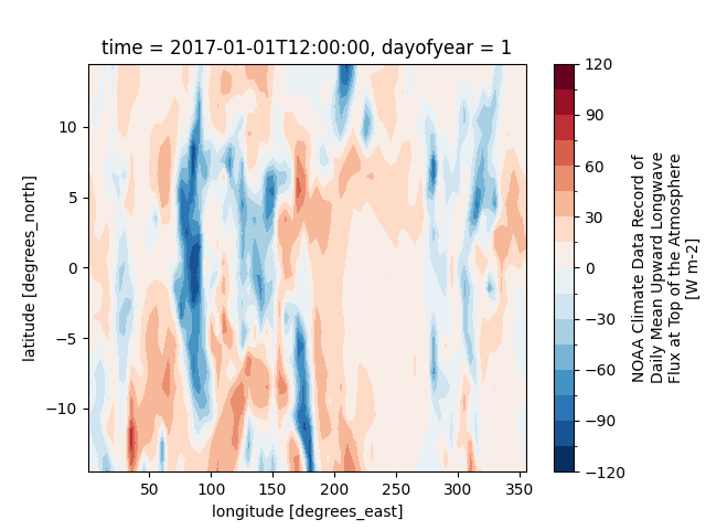
<matplotlib.contour.QuadContourSet object at 0x7ff9e41bcc70>

Separation of symmetric and asymmetric parts

data_as = ecl.field.equatorial_wave.decompose_symasym(data_dt)
data_as.isel(time = 0).plot.contourf(levels = 21)

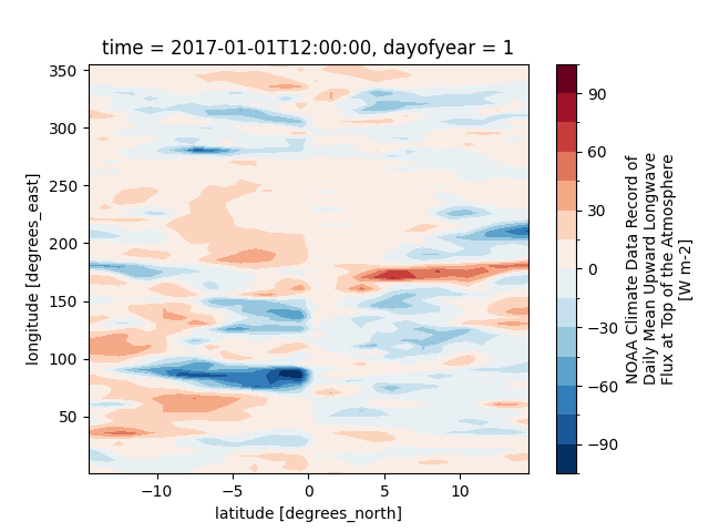
<matplotlib.contour.QuadContourSet object at 0x7ff9e1ffc130>

Calculation of spectral coefficients

psum = ecl.field.equatorial_wave.calc_spectral_coefficients(data_as,spd,nDayWin,nDaySkip)
psum

<xarray.Dataset> Size: 24kB
Dimensions:     (freq: 48, k: 31)
Coordinates:
  * freq        (freq) float64 384B 0.01042 0.02083 0.03125 ... 0.4896 0.5
  * k           (k) float64 248B -15.0 -14.0 -13.0 -12.0 ... 12.0 13.0 14.0 15.0
Data variables:
    psumanti_r  (freq, k) float64 12kB nan nan nan nan ... 1.059 0.939 0.8096
    psumsym_r   (freq, k) float64 12kB nan nan nan nan ... 1.124 1.076 1.15

xarray.Dataset

• Dimensions:
  • freq: 48
  • k: 31
• Coordinates: (2)
  • freq
    (freq)
    float64
    0.01042 0.02083 ... 0.4896 0.5

    array([0.010417, 0.020833, 0.03125 , 0.041667, 0.052083, 0.0625  , 0.072917,
           0.083333, 0.09375 , 0.104167, 0.114583, 0.125   , 0.135417, 0.145833,
           0.15625 , 0.166667, 0.177083, 0.1875  , 0.197917, 0.208333, 0.21875 ,
           0.229167, 0.239583, 0.25    , 0.260417, 0.270833, 0.28125 , 0.291667,
           0.302083, 0.3125  , 0.322917, 0.333333, 0.34375 , 0.354167, 0.364583,
           0.375   , 0.385417, 0.395833, 0.40625 , 0.416667, 0.427083, 0.4375  ,
           0.447917, 0.458333, 0.46875 , 0.479167, 0.489583, 0.5     ])

  • k
    (k)
    float64
    -15.0 -14.0 -13.0 ... 14.0 15.0

    array([-15., -14., -13., -12., -11., -10.,  -9.,  -8.,  -7.,  -6.,  -5.,  -4.,
            -3.,  -2.,  -1.,   0.,   1.,   2.,   3.,   4.,   5.,   6.,   7.,   8.,
             9.,  10.,  11.,  12.,  13.,  14.,  15.])

• Data variables: (2)
  • psumanti_r
    (freq, k)
    float64
    nan nan nan ... 1.059 0.939 0.8096

    array([[       nan,        nan,        nan, ...,        nan,        nan,
                   nan],
           [0.92061326, 0.88245882, 1.03744306, ..., 1.09548578, 1.11793649,
            0.9712682 ],
           [0.94331562, 0.89904479, 1.00798604, ..., 1.05584688, 1.10163394,
            1.05019981],
           ...,
           [1.05520495, 0.93362824, 0.89149815, ..., 1.05094287, 0.93405879,
            0.9132496 ],
           [0.9709381 , 0.94903587, 0.9647387 , ..., 1.10711583, 0.86811829,
            0.85635997],
           [0.83049446, 0.96880045, 0.99744281, ..., 1.05923972, 0.93904522,
            0.80964553]], shape=(48, 31))

  • psumsym_r
    (freq, k)
    float64
    nan nan nan ... 1.124 1.076 1.15

    array([[       nan,        nan,        nan, ...,        nan,        nan,
                   nan],
           [0.95145217, 0.87353509, 1.21584265, ..., 1.35959477, 1.11485602,
            1.09621416],
           [1.01113478, 1.00279496, 1.38343632, ..., 1.22498064, 1.01795419,
            1.20603809],
           ...,
           [1.00233878, 1.11887196, 1.12901098, ..., 1.14873035, 1.21045733,
            1.27666735],
           [1.04611579, 1.09378167, 1.12991273, ..., 1.15898716, 1.1583915 ,
            1.16781296],
           [1.12293724, 1.05945028, 1.1084282 , ..., 1.12382697, 1.07578409,
            1.15010604]], shape=(48, 31))

• Indexes: (2)
  • freq
    PandasIndex

    PandasIndex(Index([0.010416666666666666, 0.020833333333333332,              0.03125,
           0.041666666666666664, 0.052083333333333336,               0.0625,
            0.07291666666666667,  0.08333333333333333,              0.09375,
            0.10416666666666667,  0.11458333333333333,                0.125,
            0.13541666666666666,  0.14583333333333334,              0.15625,
            0.16666666666666666,  0.17708333333333334,               0.1875,
            0.19791666666666666,  0.20833333333333334,              0.21875,
            0.22916666666666666,  0.23958333333333334,                 0.25,
             0.2604166666666667,   0.2708333333333333,              0.28125,
             0.2916666666666667,   0.3020833333333333,               0.3125,
             0.3229166666666667,   0.3333333333333333,              0.34375,
             0.3541666666666667,   0.3645833333333333,                0.375,
             0.3854166666666667,   0.3958333333333333,              0.40625,
             0.4166666666666667,   0.4270833333333333,               0.4375,
             0.4479166666666667,   0.4583333333333333,              0.46875,
             0.4791666666666667,   0.4895833333333333,                  0.5],
          dtype='float64', name='freq'))

  • k
    PandasIndex

    PandasIndex(Index([-15.0, -14.0, -13.0, -12.0, -11.0, -10.0,  -9.0,  -8.0,  -7.0,  -6.0,
            -5.0,  -4.0,  -3.0,  -2.0,  -1.0,   0.0,   1.0,   2.0,   3.0,   4.0,
             5.0,   6.0,   7.0,   8.0,   9.0,  10.0,  11.0,  12.0,  13.0,  14.0,
            15.0],
          dtype='float64', name='k'))

• Attributes: (0)

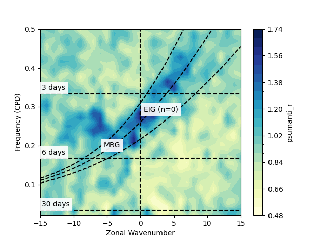
Drawing asymmetric parts

fig, ax = plt.subplots()

psum.psumanti_r.plot.contourf(ax = ax, levels=21, cmap = 'YlGnBu')
ecl.field.equatorial_wave.draw_wk_anti_analysis()

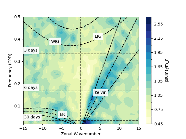
And drawing symmetric parts

fig, ax = plt.subplots()

psum.psumsym_r.plot.contourf(ax = ax, levels=21, cmap = 'YlGnBu')
ecl.field.equatorial_wave.draw_wk_sym_analysis()