Potential Intensity for Typhoon

Potential Intensity for Typhoon#

Before proceeding with all the steps, first import some necessary libraries and packages

import xarray as xr
import cartopy.crs as ccrs
import easyclimate as ecl

Now open the sample dataset

Tip

You can download following datasets here:

Download tcpi_sample_data.nc (243 kB)

ds = xr.open_dataset('tcpi_sample_data.nc')
ds

And then we use easyclimate.field.typhoon.calc_potential_intensity_Bister_Emanuel_2002 to calculate relative variables about potential intensity for typhoon

pi_result = ecl.field.typhoon.calc_potential_intensity_Bister_Emanuel_2002(
    sst_data = ds.sst,
    sst_data_units = 'degC',
    surface_pressure_data = ds.msl,
    surface_pressure_data_units = 'hPa',
    temperature_data = ds.t,
    temperature_data_units = 'degC',
    specific_humidity_data = ds.q,
    specific_humidity_data_units = 'g/kg',
    vertical_dim = 'level',
    vertical_dim_units = 'hPa'
)
pi_result

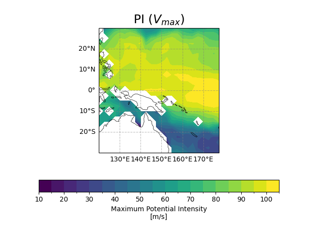
Potential Intensity (PI, $V_{max}$)#

fig, ax = ecl.plot.quick_draw_spatial_basemap(central_longitude = 200)
pi_result.vmax.plot.contourf(
    ax = ax,
    cbar_kwargs = {'location': 'bottom'},
    transform = ccrs.PlateCarree(),
    levels = 21
)
ax.set_title('PI ($V_{max}$)', size = 18)

$PI ($V_{max}$)$

Text(0.5, 1.0, 'PI ($V_{max}$)')

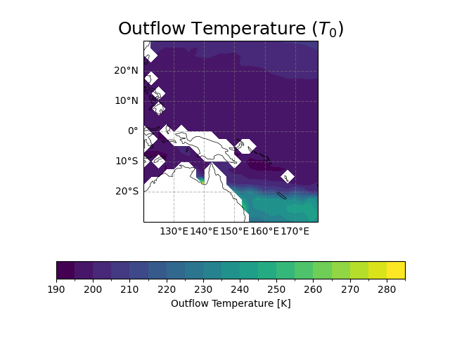
Outflow Temperature ($T_0$)#

fig, ax = ecl.plot.quick_draw_spatial_basemap(central_longitude = 200)
pi_result.t0.plot.contourf(
    ax = ax,
    cbar_kwargs = {'location': 'bottom'},
    transform = ccrs.PlateCarree(),
    levels = 21
)
ax.set_title('Outflow Temperature ($T_0$)', size = 18)

Text(0.5, 1.0, 'Outflow Temperature ($T_0$)')

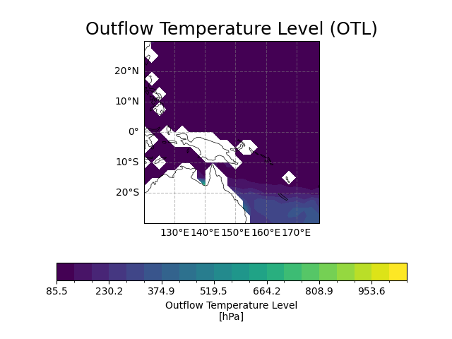
Outflow Temperature Level (OTL)#

fig, ax = ecl.plot.quick_draw_spatial_basemap(central_longitude = 200)
pi_result.otl.plot.contourf(
    ax = ax,
    cbar_kwargs = {'location': 'bottom'},
    transform = ccrs.PlateCarree(),
    vmax = 1050,
    levels =21
)
ax.set_title('Outflow Temperature Level (OTL)', size = 18)

Text(0.5, 1.0, 'Outflow Temperature Level (OTL)')

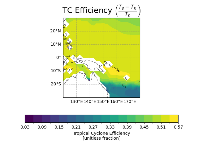
TC Efficiency ($\frac{T_{s} - T_{0}}{T_{0}}$)#

fig, ax = ecl.plot.quick_draw_spatial_basemap(central_longitude = 200)
pi_result.eff.plot.contourf(
    ax = ax,
    cbar_kwargs = {'location': 'bottom'},
    transform = ccrs.PlateCarree(),
    levels = 21
)
ax.set_title('TC Efficiency $\\left(\\frac{T_{s} - T_{0}}{T_{0}}\\right)$', size = 18)

$TC Efficiency $\left(\frac{T_{s} - T_{0}}{T_{0}}\right)$$

Text(0.5, 1.0258451865594727, 'TC Efficiency $\\left(\\frac{T_{s} - T_{0}}{T_{0}}\\right)$')

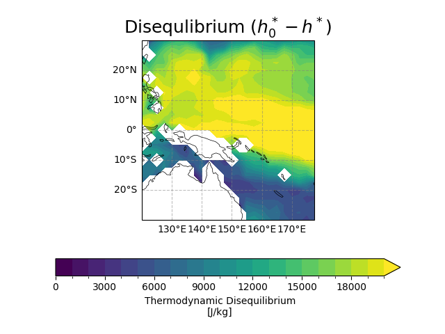
Disequlibrium ($h_0^* - h^*$)#

fig, ax = ecl.plot.quick_draw_spatial_basemap(central_longitude = 200)
pi_result.diseq.plot.contourf(
    ax = ax,
    cbar_kwargs = {'location': 'bottom'},
    transform = ccrs.PlateCarree(),
    vmin = 0,
    vmax = 20000,
    levels = 21
)
ax.set_title('Disequlibrium ($h_0^* - h^*$)', size = 18)

Text(0.5, 1.0041228612657185, 'Disequlibrium ($h_0^* - h^*$)')

Total running time of the script: (0 minutes 10.649 seconds)

Potential Intensity for Typhoon

Contents

Potential Intensity for Typhoon#

Potential Intensity (PI, \(V_{max}\))#

Outflow Temperature (\(T_0\))#

Outflow Temperature Level (OTL)#

TC Efficiency (\(\frac{T_{s} - T_{0}}{T_{0}}\))#

Disequlibrium (\(h_0^* - h^*\))#