Note
Go to the end to download the full example code.
Wet-bulb Temperature
Wet-bulb temperature is a critical meteorological parameter that represents the lowest temperature to which air can be cooled by evaporation at constant pressure. It is widely used in weather forecasting, heat stress assessment, and climate studies. The easyclimate library provides multiple methods to compute wet-bulb temperature, including iterative approaches, empirical formulas, and approximations based on established research.
The example is structured into several sections, each performing a specific task, such as data initialization, mesh grid creation, wet-bulb temperature calculations using different methods, and plotting results for analysis. The following sections describe the intent of each part.
This part imports necessary Python libraries for data manipulation and visualization:
import easyclimate as ecl
import xarray as xr
import numpy as np
import matplotlib.pyplot as plt
This section creates synthetic datasets to represent atmospheric conditions:
temp_data: A 1D array of temperatures ranging from -20°C to 50°C.relative_humidity_data: A 1D array of relative humidity values from 0% to 100%.deltaT_data: A 1D array representing the temperature difference (\(T - T_d\)) from 0°C to 30°C.
These arrays serve as input for subsequent calculations, covering a wide range of conditions to test the wet-bulb temperature methods.
temp_data = xr.DataArray(
    np.linspace(-20, 50, 71),
    dims="temp",
    coords={'temp': np.linspace(-20, 50, 71)}
)
relative_humidity_data = xr.DataArray(
    np.linspace(0, 100, 101),
    dims="rh",
    coords={'rh': np.linspace(0, 100, 101)}
)

deltaT_data = xr.DataArray(
    np.linspace(0, 30, 31),
    dims="deltaT",
    coords={'deltaT': np.linspace(0, 30, 31)}
)
This section defines the generate_mesh function, which creates 2D mesh grids from two 1D xarray.DataArray inputs. The function:
Uses numpy.meshgrid to generate grid arrays.
Constructs
xarray.DataArrayobjects for each grid, preserving coordinates and dimensions.Returns two DataArray objects representing the meshed variables.
This function is used to create 2D grids for temperature, relative humidity, and dewpoint differences, enabling calculations over a range of conditions.
def generate_mesh(
    da1: xr.DataArray,
    da2: xr.DataArray,
):
    da1_grid, da2_grid = np.meshgrid(da1, da2)

    dim_1 = da2.dims[0]
    dim_2 = da1.dims[0]
    dim_1_array = da2[dim_1].data
    dim_2_array = da1[dim_2].data

    da1_dataarray = xr.DataArray(
        da1_grid,
        dims=(dim_1, dim_2),
        coords={dim_1: dim_1_array, dim_2: dim_2_array}
    )
    da1_dataarray.name = dim_2

    da2_dataarray = xr.DataArray(
        da2_grid,
        dims=(dim_1, dim_2),
        coords={dim_1: dim_1_array, dim_2: dim_2_array}
    )
    da2_dataarray.name = dim_1

    return da1_dataarray, da2_dataarray
This section applies the generate_mesh function to create 2D grids:
temp_mesh1, rh_mesh: Meshes of temperature and relative humidity.
temp_mesh2, deltaT_mesh: Meshes of temperature and temperature difference.
td_mesh: Dewpoint temperature calculated as temp_mesh2 - deltaT_mesh.
These grids are used as inputs for wet-bulb temperature calculations.
temp_mesh1, rh_mesh = generate_mesh(temp_data, relative_humidity_data)
temp_mesh2, deltaT_mesh = generate_mesh(temp_data, deltaT_data)
td_mesh = temp_mesh2 - deltaT_mesh
Iterative Calculation
This section computes wet-bulb potential temperature using the easyclimate.physics.calc_wet_bulb_potential_temperature_iteration
function from easyclimate. The function:
Takes temperature, relative humidity, and pressure (1013.25 hPa) as inputs.
Uses an iterative approach based on the psychrometric formula with a psychrometer constant (\(A = 0.662 \cdot 10^{-3}\)).
Outputs wet-bulb temperature in °C for a 2D grid of conditions.
See also
Fan, J. (1987). Determination of the Psychrometer Coefficient A of the WMO Reference Psychrometer by Comparison with a Standard Gravimetric Hygrometer. Journal of Atmospheric and Oceanic Technology, 4(1), 239-244. https://journals.ametsoc.org/view/journals/atot/4/1/1520-0426_1987_004_0239_dotpco_2_0_co_2.xml
Wang Haijun. (2011). Two Wet-Bulb Temperature Estimation Methods and Error Analysis. Meteorological Monthly (Chinese), 37(4): 497-502. website: http://qxqk.nmc.cn/html/2011/4/20110415.html
Cheng Zhi, Wu Biwen, Zhu Baolin, et al, (2011). Wet-Bulb Temperature Looping Iterative Scheme and Its Application. Meteorological Monthly (Chinese), 37(1): 112-115. website: http://qxqk.nmc.cn/html/2011/1/20110115.html
The result, wet_bulb_iteration, is extracted for a single pressure level.
wet_bulb_iteration = ecl.physics.calc_wet_bulb_potential_temperature_iteration(
    temp_mesh1,
    rh_mesh,
    xr.DataArray([1013.25], dims="p"),
    "degC", "%", "hPa",
    A = 0.662* 10 ** (-3),
).isel(p = 0)
wet_bulb_iteration
Stull (2011) Calculation
Single Point
This section tests the easyclimate.physics.calc_wet_bulb_temperature_stull2011 function for a single data point (T = 20°C, RH = 50%):
Computes wet-bulb temperature using Stull’s empirical formula.
Converts the result from Kelvin to Celsius for consistency.
See also
Stull, R. (2011). Wet-Bulb Temperature from Relative Humidity and Air Temperature. Journal of Applied Meteorology and Climatology, 50(11), 2267-2269. https://doi.org/10.1175/JAMC-D-11-0143.1
Stull, R. (2011): Meteorology for Scientists and Engineers. 3rd ed. Discount Textbooks, 924 pp. [Available online at https://www.eoas.ubc.ca/books/Practical_Meteorology/, https://www.eoas.ubc.ca/courses/atsc201/MSE3.html]
Knox, J. A., Nevius, D. S., & Knox, P. N. (2017). Two Simple and Accurate Approximations for Wet-Bulb Temperature in Moist Conditions, with Forecasting Applications. Bulletin of the American Meteorological Society, 98(9), 1897-1906. https://doi.org/10.1175/BAMS-D-16-0246.1
This serves as a simple validation of the Stull method before applying it to the full grid.
wet_bulb_temp_K = ecl.physics.calc_wet_bulb_temperature_stull2011(
    temperature_data = xr.DataArray([20]),
    relative_humidity_data = xr.DataArray([50]),
    temperature_data_units = "degC",
    relative_humidity_data_units = "%"
)
ecl.transfer_data_temperature_units(wet_bulb_temp_K, "K", "degC")
Grid
This section applies easyclimate.physics.calc_wet_bulb_temperature_stull2011 to the 2D grid (temp_mesh1, rh_mesh):
Calculates wet-bulb temperature across the grid using Stull’s formula.
Converts the output from Kelvin to Celsius.
Stores the result in
wet_bulb_stull2011.
This enables comparison with the iterative method.
wet_bulb_stull2011 = ecl.physics.calc_wet_bulb_temperature_stull2011(
    temp_mesh1, rh_mesh, "degC", "%"
)
wet_bulb_stull2011 = ecl.transfer_data_temperature_units(wet_bulb_stull2011, "K", "degC")
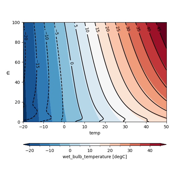
Comparison (Iteration vs. Stull)
This section visualizes the results of the iterative and Stull methods:
Creates a contour plot of wet_bulb_iteration with levels from -20°C to 50°C.
Overlays contours of wet_bulb_stull2011 in black for comparison.
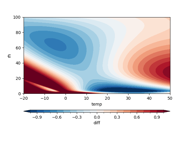
Computes and plots the difference (wet_bulb_stull2011 - wet_bulb_iteration) to highlight discrepancies.
The plots help assess the agreement between the two methods across different conditions.
fig, ax = plt.subplots(figsize = (6, 6))

wet_bulb_iteration.plot.contourf(
    levels = np.arange(-20, 50, 5),
    cbar_kwargs = {'location': 'bottom', 'aspect': 60}
)

cf = wet_bulb_stull2011.plot.contour(levels = np.arange(-20, 50, 5), colors='k')
plt.clabel(cf, inline = True, fontsize = 10)
<a list of 14 text.Text objects>
diff = (wet_bulb_stull2011 - wet_bulb_iteration)
diff.plot.contourf(
    levels = np.linspace(-1, 1, 21),
    cbar_kwargs = {'location': 'bottom', 'aspect': 60, 'label': 'diff'}
)
<matplotlib.contour.QuadContourSet object at 0x7f77d28d5210>
Sadeghi (2013) Calculation
Grid
This section computes wet-bulb temperature using easyclimate.physics.calc_wet_bulb_temperature_sadeghi2013 at three elevations (0 m, 2000 m, 5000 m):
Uses temp_mesh1 and rh_mesh as inputs, with height specified as an
xarray.DataArray.Outputs results in °C for each elevation.
See also
Sadeghi, S., Peters, T. R., Cobos, D. R., Loescher, H. W., & Campbell, C. S. (2013). Direct Calculation of Thermodynamic Wet-Bulb Temperature as a Function of Pressure and Elevation. Journal of Atmospheric and Oceanic Technology, 30(8), 1757-1765. https://doi.org/10.1175/JTECH-D-12-00191.1
This evaluates the impact of elevation on wet-bulb temperature using Sadeghi’s empirical formula.
wet_bulb_sadeghi2013_0m = ecl.physics.calc_wet_bulb_temperature_sadeghi2013(
    temp_mesh1, xr.DataArray([0], dims="height"), rh_mesh, "degC", "m", "%"
).isel(height = 0)

wet_bulb_sadeghi2013_2000m = ecl.physics.calc_wet_bulb_temperature_sadeghi2013(
    temp_mesh1, xr.DataArray([2000], dims="height"), rh_mesh, "degC", "m", "%"
).isel(height = 0)

wet_bulb_sadeghi2013_5000m = ecl.physics.calc_wet_bulb_temperature_sadeghi2013(
    temp_mesh1, xr.DataArray([5000], dims="height"), rh_mesh, "degC", "m", "%"
).isel(height = 0)
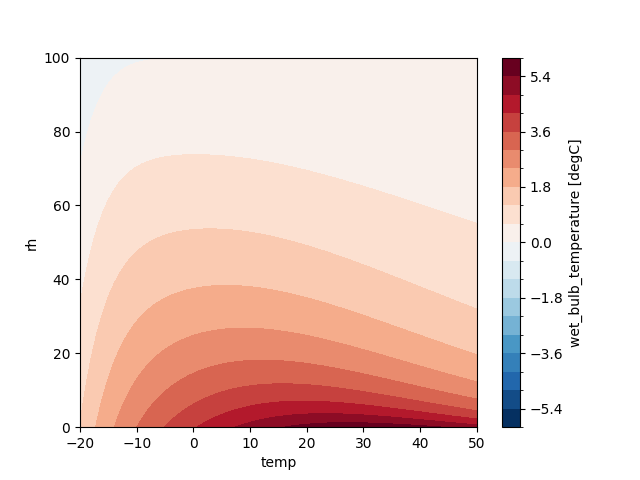
Comparison (0 m vs. 5000 m)
This section visualizes the Sadeghi results:
Creates a contour plot of
wet_bulb_sadeghi2013_0m.Overlays contours of
wet_bulb_sadeghi2013_5000min black.Plots the difference (
wet_bulb_sadeghi2013_0m - wet_bulb_sadeghi2013_5000m) to show elevation effects.
These plots illustrate how elevation influences wet-bulb temperature.
wet_bulb_sadeghi2013_0m.plot.contourf(levels = 21)
wet_bulb_sadeghi2013_5000m.plot.contour(levels = 21, colors='k')
<matplotlib.contour.QuadContourSet object at 0x7f77d2960bd0>
diff = wet_bulb_sadeghi2013_0m - wet_bulb_sadeghi2013_5000m
diff.plot.contourf(
    levels = np.linspace(-6, 6, 21)
)
<matplotlib.contour.QuadContourSet object at 0x7f77d1d21b10>
Davies-Jones (2008) Calculation
Grid
This section computes wet-bulb potential temperature using easyclimate.physics.calc_wet_bulb_potential_temperature_davies_jones2008:
Uses
temp_mesh2,td_mesh, and a pressure of 1000 hPa as inputs.Converts the output from Kelvin to Celsius.
Stores the result in
wet_bulb_davies_jones2008.
See also
Davies-Jones, R. (2008). An Efficient and Accurate Method for Computing the Wet-Bulb Temperature along Pseudoadiabats. Monthly Weather Review, 136(7), 2764-2785. https://doi.org/10.1175/2007MWR2224.1
Knox, J. A., Nevius, D. S., & Knox, P. N. (2017). Two Simple and Accurate Approximations for Wet-Bulb Temperature in Moist Conditions, with Forecasting Applications. Bulletin of the American Meteorological Society, 98(9), 1897-1906. https://doi.org/10.1175/BAMS-D-16-0246.1
This applies Davies-Jones’ approximation, which uses dewpoint temperature directly.
wet_bulb_davies_jones2008 = ecl.physics.calc_wet_bulb_potential_temperature_davies_jones2008(
    pressure_data = xr.DataArray([1000], dims = "p"), temperature_data = temp_mesh2, dewpoint_data = td_mesh,
    pressure_data_units = "hPa", temperature_data_units = "degC", dewpoint_data_units = "degC",
).isel(p = 0)
wet_bulb_davies_jones2008 = ecl.transfer_data_temperature_units(wet_bulb_davies_jones2008, "K", "degC")
wet_bulb_davies_jones2008
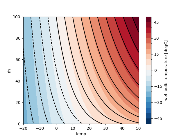
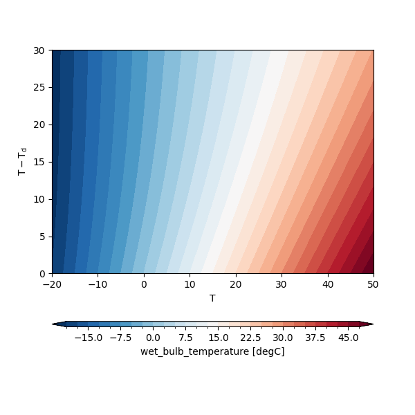
Plot Davies-Jones Results
This section visualizes the Davies-Jones results:
Creates a contour plot of wet_bulb_davies_jones2008 with levels from -20°C to 50°C.
Labels axes with temperature (\(T\)) and temperature-dewpoint difference (\(T - T_d\)).
This plot provides insight into the behavior of the Davies-Jones method across the grid.
fig, ax = plt.subplots(figsize = (6, 6))

wet_bulb_davies_jones2008.plot.contourf(
    levels = np.arange(-20, 50, 2.5),
    cbar_kwargs = {'location': 'bottom', 'aspect': 60}
)
ax.set_xlabel("$\\mathrm{T}$")
ax.set_ylabel("$\\mathrm{T - T_d}$")
Text(42.097222222222214, 0.5, '$\\mathrm{T - T_d}$')
Conclusion
The example demonstrates the application of multiple wet-bulb temperature calculation methods provided by the easyclimate library. By generating synthetic data, creating 2D grids, and applying iterative, empirical, and approximation-based methods, the script enables a comprehensive comparison of results. Visualizations highlight differences between methods and the influence of parameters like elevation, aiding in the evaluation of their accuracy and applicability in meteorological analysis.
Total running time of the script: (0 minutes 13.475 seconds)