Note
Go to the end to download the full example code.
Ocean Surface Mixed Layers Analysis#
Before proceeding with all the steps, first import some necessary libraries and packages
import xarray as xr
import numpy as np
import matplotlib.pyplot as plt
import easyclimate as ecl
Preprocessed data
temper_data = xr.open_dataset('temp_soda3.4.2_mn_ocean_reg_2020_EN4.nc', chunks="auto").temp.rename({'st_ocean': 'depth'})
slt_data = xr.open_dataset('salt_soda3.4.2_mn_ocean_reg_2020_EN4.nc', chunks="auto").salt.rename({'st_ocean': 'depth'})

u_data = xr.open_dataset('u_soda3.4.2_mn_ocean_reg_2020_EN4.nc', chunks="auto").u.rename({'st_ocean': 'depth'})
v_data = xr.open_dataset('v_soda3.4.2_mn_ocean_reg_2020_EN4.nc', chunks="auto").v.rename({'st_ocean': 'depth'})
net_heating_data = xr.open_dataset('net_heating_soda3.4.2_mn_ocean_reg_2020_EN4.nc', chunks="auto").net_heating

wt_data = xr.open_dataset('wt_soda3.4.2_mn_ocean_reg_2020_EN4.nc', chunks="auto").wt.rename({'sw_ocean': 'depth'})
The following data is the depth data of the mixed layer output by the oceanic models (we will compare it with it later).
mld_data = xr.open_dataset('mlp_soda3.4.2_mn_ocean_reg_2020_EN4.nc', chunks="auto").mlp
Tip
You can download following datasets here:
Warning
Here we are using only the SODA 3.4.2 reanalysis data during 2024; the actual analysis will need to be analyzed using multiple years of data and removing the seasonal cycle by
easyclimate.remove_seasonal_cycle_mean.Citation: Carton, J. A., Chepurin, G. A., & Chen, L. (2018). SODA3: A New Ocean Climate Reanalysis. Journal of Climate, 31(17), 6967-6983. https://doi.org/10.1175/JCLI-D-18-0149.1
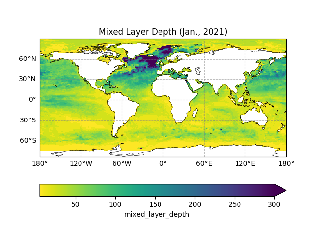
Mix-Layer Depth#
Here, we use easyclimate.field.ocean.calc_mixed_layer_depth to calculate the depth of mix-layer (MLD).
mixed_layer_depth = ecl.field.ocean.calc_mixed_layer_depth(
    seawater_temperature_data = temper_data,
    seawater_practical_salinity_data = slt_data,
).to_netcdf("sample_mixed_layer_depth.nc")
Next, we open the dataset containing the results
mixed_layer_depth = xr.open_dataarray("sample_mixed_layer_depth.nc")
mixed_layer_depth
Draw the figure of mix-layer depth
fig, ax = ecl.plot.quick_draw_spatial_basemap()

mixed_layer_depth.isel(time = 0).plot(
    vmax = 300,
    cmap = "viridis_r",
    cbar_kwargs = {'location': 'bottom'},
)
ax.set_title("Mixed Layer Depth (Jan., 2021)")
Text(0.5, 1.0, 'Mixed Layer Depth (Jan., 2021)')
Compare with the depth data of the mixed layer output by the oceanic models
fig, ax = ecl.plot.quick_draw_spatial_basemap()
diff = mld_data.isel(time = 0) - mixed_layer_depth.isel(time = 0)
diff.plot(
    vmax = 200,
    cbar_kwargs = {'location': 'bottom', 'label': 'units: m'},
)
ax.set_title("SODA minus Easyclimate (pyoceans)")
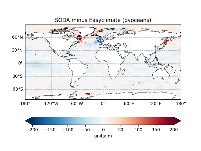
Text(0.5, 1.0, 'SODA minus Easyclimate (pyoceans)')
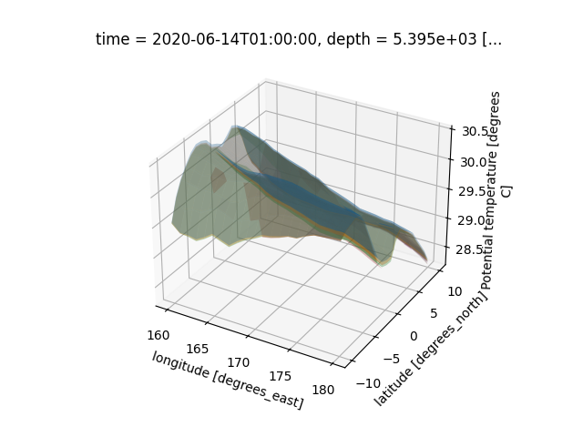
MLD Internal Temperature#
We use easyclimate.field.ocean.get_temper_within_MLD to receive MLD internal temperature.
mld_t = ecl.field.ocean.get_temper_within_MLD(
    seawater_temperature_data = temper_data,
    mixed_layer_depth = mld_data,
).to_netcdf("sample_mld_t.nc")
Next, we open the dataset containing the results
mld_t = xr.open_dataarray("sample_mld_t.nc")
mld_t
Now, Plotting the temperature of a marine model layer within a mixed layer
ax = plt.figure().add_subplot(projection='3d')

for depth_value in np.arange(50):
    mld_t.isel(time = 5).sel(lon = slice(160, 180), lat = slice(-10, 10)).isel(depth = depth_value).plot.surface(
        alpha=0.3,
    )
MLD Internal Average Temperature#
We use easyclimate.field.ocean.calc_MLD_depth_weighted to calculate MLD internal average temperature.
weight = ecl.field.ocean.calc_MLD_depth_weighted(
    seawater_temperature_data = temper_data,
    mixed_layer_depth = mld_data
)

mld_t_ave = ecl.field.ocean.get_data_average_within_MLD(
    data_input = temper_data,
    mixed_layer_depth = mld_data,
    depth_weight = weight
).to_netcdf("sample_mld_t_ave.nc")
Warning
You can NOT use above result (i.e., mld_t) to directly calculate MLD internal average temperature by mld_t.mean(dim = "depth"), because the vertical layers in ocean models are usually not uniformly distributed.
Next, we open the dataset containing the results
mld_t_ave = xr.open_dataarray("sample_mld_t_ave.nc")
mld_t_ave
Now, Plotting the MLD internal average temperature
fig, ax = ecl.plot.quick_draw_spatial_basemap()

mld_t_ave.isel(time = 0).plot.contourf(
    levels = 21,
    cbar_kwargs = {'location': 'bottom', 'label': 'degC'},
)
ax.set_title("Mixed Layer Temperature (Jan., 2021)")
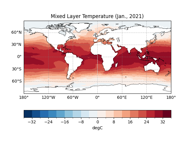
Text(0.5, 1.0, 'Mixed Layer Temperature (Jan., 2021)')
MLD Average Temperature Tendency#
We use easyclimate.field.ocean.calc_MLD_temper_tendency to calculate MLD internal average temperature tendency.
weight = ecl.field.ocean.calc_MLD_depth_weighted(
    seawater_temperature_data = temper_data,
    mixed_layer_depth = mld_data
)

mld_t_tendency = ecl.field.ocean.calc_MLD_temper_tendency(
    seawater_temperature_anomaly_data = temper_data,
    mixed_layer_depth = mld_data,
    depth_weight = weight
).to_netcdf("sample_mld_t_tendency.nc")
mld_t_tendency = xr.open_dataarray("sample_mld_t_tendency.nc")
mld_t_tendency
Now, Plotting the result.
fig, ax = ecl.plot.quick_draw_spatial_basemap()

mld_t_tendency.isel(time = 5).plot.contourf(
    vmax = 8,
    levels = 21,
    cbar_kwargs = {'location': 'bottom'},
)
ax.set_title("Mixed Layer Temperature Tendency (Jun., 2021)")
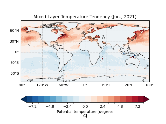
Text(0.5, 1.0, 'Mixed Layer Temperature Tendency (Jun., 2021)')
MLD Average Horizontal Advection#
We use easyclimate.field.ocean.calc_MLD_average_horizontal_advection to calculate MLD average horizontal advection.
weight = ecl.field.ocean.calc_MLD_depth_weighted(
    seawater_temperature_data = temper_data,
    mixed_layer_depth = mld_data
)

mld_horizontal_advection = ecl.field.ocean.calc_MLD_average_horizontal_advection(
    u_monthly_data = u_data,
    v_monthly_data = v_data,
    seawater_temperature_data = temper_data,
    mixed_layer_depth = mld_data,
    depth_weight = weight
).to_netcdf("sample_mld_horizontal_advection.nc")
mld_horizontal_advection = xr.open_dataset("sample_mld_horizontal_advection.nc")
Now, Plotting the result for zonal advection.
fig, ax = ecl.plot.quick_draw_spatial_basemap()

mld_horizontal_advection["u_advection"].isel(time = 5).plot(
    vmax = 2,
    levels = 21,
    cbar_kwargs = {'location': 'bottom'},
)
ax.set_title("Mixed Layer U advection (Jun., 2021)")
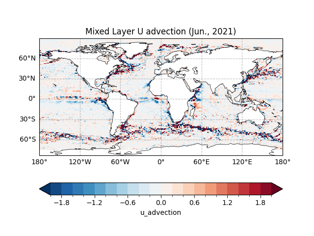
Text(0.5, 1.0, 'Mixed Layer U advection (Jun., 2021)')
And meridional advection.
fig, ax = ecl.plot.quick_draw_spatial_basemap()

mld_horizontal_advection["v_advection"].isel(time = 5).plot(
    vmax = 2,
    levels = 21,
    cbar_kwargs = {'location': 'bottom'},
)
ax.set_title("Mixed Layer V advection (Jun., 2021)")
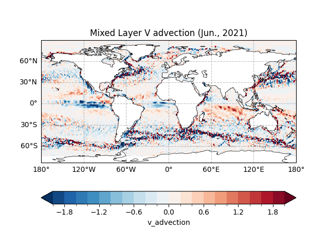
Text(0.5, 1.0, 'Mixed Layer V advection (Jun., 2021)')
MLD Average Vertical Advection#
We use easyclimate.field.ocean.calc_MLD_average_vertical_advection to calculate MLD average vertical advection.
weight = ecl.field.ocean.calc_MLD_depth_weighted(
    seawater_temperature_data = temper_data,
    mixed_layer_depth = mld_data
)

mld_vertical_advection = ecl.field.ocean.calc_MLD_average_vertical_advection(
    w_monthly_data = wt_data,
    seawater_temperature_data = temper_data,
    mixed_layer_depth = mld_data,
    depth_weight = weight
).to_netcdf("sample_mld_vertical_advection.nc")
mld_vertical_advection = xr.open_dataarray("sample_mld_vertical_advection.nc")
mld_vertical_advection
Now, Plotting the result.
fig, ax = ecl.plot.quick_draw_spatial_basemap()

mld_vertical_advection.isel(time = 5).plot(
    vmax = 2,
    levels = 21,
    cbar_kwargs = {'location': 'bottom'},
)
ax.set_title("Mixed Layer vertical advection (Jun., 2021)")
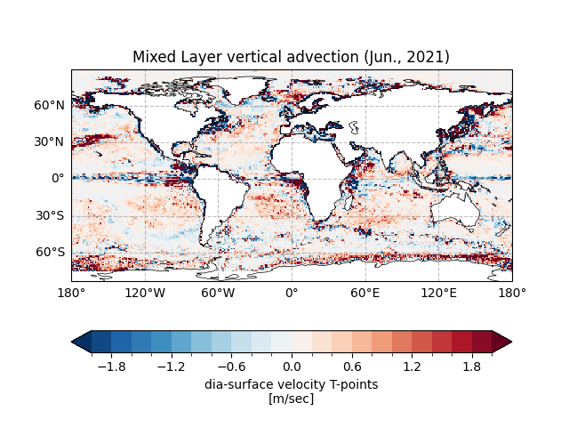
Text(0.5, 1.0, 'Mixed Layer vertical advection (Jun., 2021)')
Surface Heat Flux#
We use easyclimate.field.ocean.calc_ocean_surface_heat_flux to calculate ocean surface heat flux.
surface_heat_flux = ecl.field.ocean.calc_ocean_surface_heat_flux(
    qnet_monthly_anomaly_data = net_heating_data,
    mixed_layer_depth = mld_data,
).to_netcdf("sample_surface_heat_flux.nc")
surface_heat_flux = xr.open_dataarray("sample_surface_heat_flux.nc")
surface_heat_flux
Now, Plotting the result.
fig, ax = ecl.plot.quick_draw_spatial_basemap()

surface_heat_flux.isel(time = 5).plot(
    vmax = 10,
    levels = 21,
    cbar_kwargs = {'location': 'bottom'},
)
ax.set_title("Surface Heat Flux (Jun., 2021)")
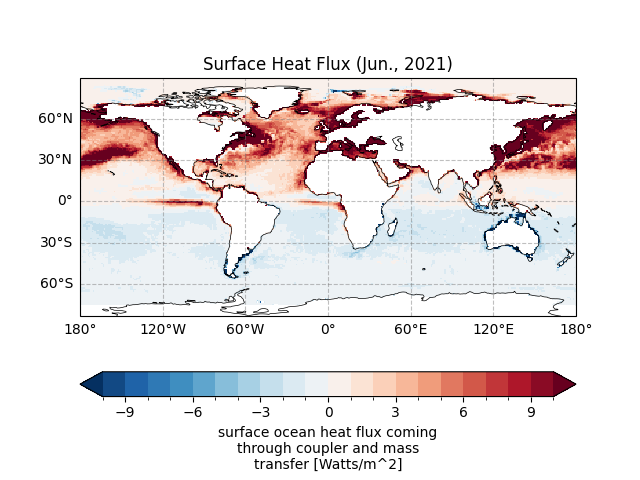
Text(0.5, 1.0, 'Surface Heat Flux (Jun., 2021)')
Total running time of the script: (0 minutes 17.200 seconds)