Note
Go to the end to download the full example code.
Empirical Orthogonal Function (EOF) and Maximum Covariance Analysis (MCA)#
Before proceeding with all the steps, first import some necessary libraries and packages
import xarray as xr
import easyclimate as ecl
import matplotlib.pyplot as plt
import cartopy.crs as ccrs
Empirical Orthogonal Function#
Read raw precipitation and temperature data
t_data = xr.open_dataset("t_ERA5_1982-2022_N80.nc").t.sel(time = slice("1982-01-01", "2020-12-31")).sortby("lat")
precip_data = xr.open_dataset("precip_ERA5_1982-2020_N80.nc").precip.sel(time = slice("1982-01-01", "2020-12-31")).sortby("lat")
Tip
You can download following datasets here:
Be limited to the East Asia region and conduct empirical orthogonal function (EOF) analysis on it
precip_data_EA = precip_data.sel(lon = slice(105, 130), lat = slice(20, 40))
model = ecl.eof.get_EOF_model(precip_data_EA, lat_dim = 'lat', lon_dim = 'lon', remove_seasonal_cycle_mean = True, use_coslat = True)
eof_analysis_result = ecl.eof.calc_EOF_analysis(model)
eof_analysis_result.to_netcdf("eof_analysis_result.nc")
Load the analyzed data
eof_analysis_result = xr.open_dataset("eof_analysis_result.nc")
eof_analysis_result
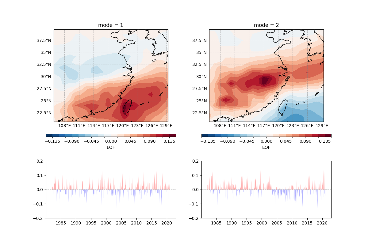
Draw the leading first and second modes
fig = plt.figure(figsize = (12, 8))
fig.subplots_adjust(hspace = 0.15, wspace = 0.2)
gs = fig.add_gridspec(3, 2)

proj = ccrs.PlateCarree(central_longitude = 200)
proj_trans = ccrs.PlateCarree()

axi = fig.add_subplot(gs[0:2, 0], projection = proj)
draw_data = eof_analysis_result["EOF"].sel(mode = 1)
draw_data.plot.contourf(
    ax = axi, levels = 21,
    transform = proj_trans,
    cbar_kwargs={"location": "bottom", "aspect": 50, "pad" : 0.1}
)
axi.coastlines()
axi.gridlines(draw_labels=["left", "bottom"], color="grey", alpha=0.5, linestyle="--")

axi = fig.add_subplot(gs[2, 0])
ecl.plot.line_plot_with_threshold(eof_analysis_result["PC"].sel(mode = 1), line_plot=False)
axi.set_ylim(-0.2, 0.2)

axi = fig.add_subplot(gs[0:2, 1], projection = proj)
draw_data = eof_analysis_result["EOF"].sel(mode = 2)
draw_data.plot.contourf(
    ax = axi, levels = 21,
    transform = proj_trans,
    cbar_kwargs={"location": "bottom", "aspect": 50, "pad" : 0.1}
)
axi.coastlines()
axi.gridlines(draw_labels=["left", "bottom"], color="grey", alpha=0.5, linestyle="--")

axi = fig.add_subplot(gs[2, 1])
ecl.plot.line_plot_with_threshold(eof_analysis_result["PC"].sel(mode = 2), line_plot=False)
axi.set_ylim(-0.2, 0.2)
(-0.2, 0.2)
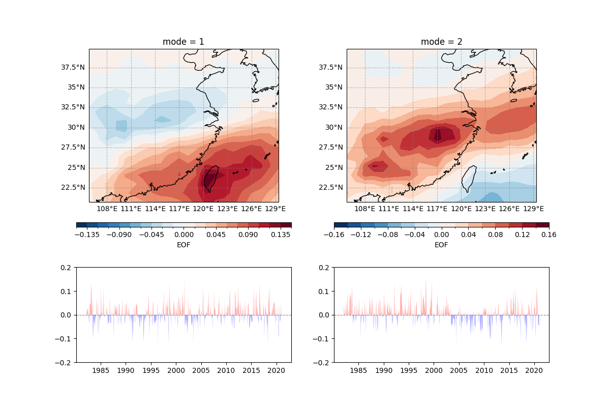
Rotated Empirical Orthogonal Function#
Here, we conduct rotated empirical orthogonal function (REOF) analysis on it
model = ecl.eof.get_REOF_model(precip_data_EA, lat_dim = 'lat', lon_dim = 'lon', remove_seasonal_cycle_mean = True, use_coslat = True)
reof_analysis_result = ecl.eof.calc_REOF_analysis(model)
reof_analysis_result.to_netcdf("reof_analysis_result.nc")
Now load the data
reof_analysis_result = xr.open_dataset("reof_analysis_result.nc")
reof_analysis_result
fig = plt.figure(figsize = (12, 8))
fig.subplots_adjust(hspace = 0.15, wspace = 0.2)
gs = fig.add_gridspec(3, 2)

proj = ccrs.PlateCarree(central_longitude = 200)
proj_trans = ccrs.PlateCarree()

axi = fig.add_subplot(gs[0:2, 0], projection = proj)
draw_data = reof_analysis_result["EOF"].sel(mode = 1)
draw_data.plot.contourf(
    ax = axi, levels = 21,
    transform = proj_trans,
    cbar_kwargs={"location": "bottom", "aspect": 50, "pad" : 0.1}
)
axi.coastlines()
axi.gridlines(draw_labels=["left", "bottom"], color="grey", alpha=0.5, linestyle="--")

axi = fig.add_subplot(gs[2, 0])
ecl.plot.line_plot_with_threshold(reof_analysis_result["PC"].sel(mode = 1), line_plot=False)
axi.set_ylim(-0.2, 0.2)

axi = fig.add_subplot(gs[0:2, 1], projection = proj)
draw_data = reof_analysis_result["EOF"].sel(mode = 2)
draw_data.plot.contourf(
    ax = axi, levels = 21,
    transform = proj_trans,
    cbar_kwargs={"location": "bottom", "aspect": 50, "pad" : 0.1}
)
axi.coastlines()
axi.gridlines(draw_labels=["left", "bottom"], color="grey", alpha=0.5, linestyle="--")

axi = fig.add_subplot(gs[2, 1])
ecl.plot.line_plot_with_threshold(reof_analysis_result["PC"].sel(mode = 2), line_plot=False)
axi.set_ylim(-0.2, 0.2)
(-0.2, 0.2)
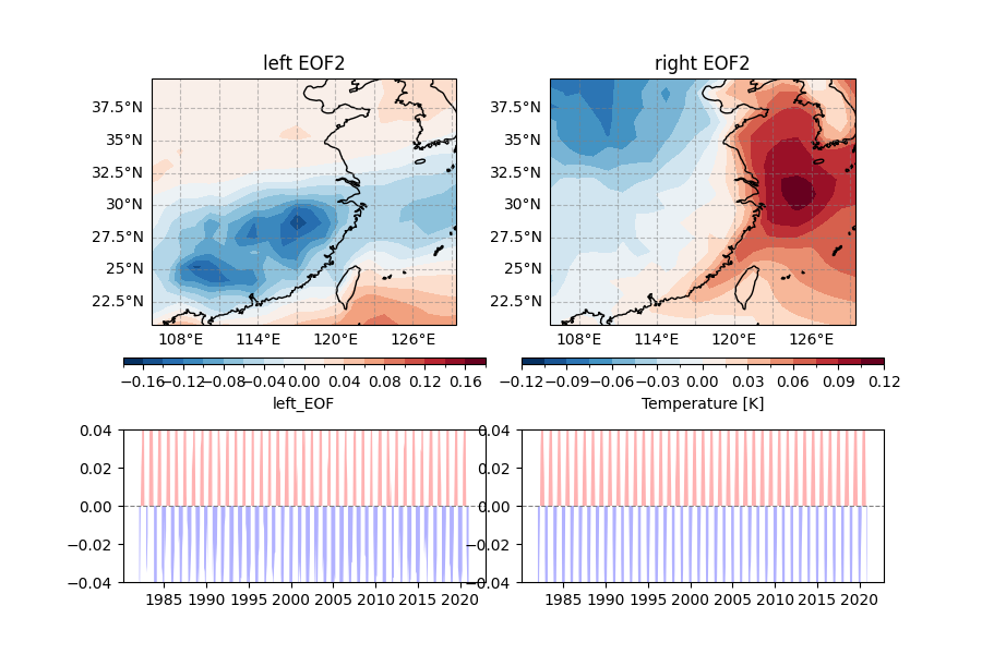
Maximum Covariance Analysis#
Be limited to the East Asia region for precipitation and temperature.
precip_data_EA = precip_data.sel(lon = slice(105, 130), lat = slice(20, 40))
t_data_EA = t_data.sel(lon = slice(105, 130), lat = slice(20, 40)).sel(level = 1000)
Maximum Covariance Analysis (MCA) between two data sets.
mca_model = ecl.eof.get_MCA_model(precip_data_EA, t_data_EA, lat_dim="lat", lon_dim="lon", n_modes=2, use_coslat=True,random_state=0)
mca_analysis_result = ecl.eof.calc_MCA_analysis(mca_model)
mca_analysis_result.to_zarr("mca_analysis_result.zarr")
Now load the data
mca_analysis_result = ecl.open_datanode("./mca_analysis_result.zarr")
mca_analysis_result
Draw results for leading modes
fig = plt.figure(figsize = (9, 6))
fig.subplots_adjust(hspace = 0.15, wspace = 0.1)
gs = fig.add_gridspec(3, 2)

proj = ccrs.PlateCarree(central_longitude = 200)
proj_trans = ccrs.PlateCarree()

# ---------------
axi = fig.add_subplot(gs[0:2, 0], projection = proj)
draw_data = mca_analysis_result["EOF/left_EOF"].sel(mode = 2).left_EOF
draw_data.plot.contourf(
    ax = axi, levels = 21,
    transform = proj_trans,
    cbar_kwargs={"location": "bottom", "aspect": 50, "pad" : 0.1}
)
axi.coastlines()
axi.gridlines(draw_labels=["left", "bottom"], color="grey", alpha=0.5, linestyle="--")
axi.set_title('left EOF2')

# ---------------
axi = fig.add_subplot(gs[2, 0])
ecl.plot.line_plot_with_threshold(mca_analysis_result["PC/left_PC"].sel(mode = 1).left_PC, line_plot=False)
axi.set_ylim(-0.04, 0.04)

# ---------------
axi = fig.add_subplot(gs[0:2, 1], projection = proj)
draw_data = mca_analysis_result["EOF/right_EOF"].sel(mode = 2).right_EOF
draw_data.plot.contourf(
    ax = axi, levels = 21,
    transform = proj_trans,
    cbar_kwargs={"location": "bottom", "aspect": 50, "pad" : 0.1}
)
axi.coastlines()
axi.gridlines(draw_labels=["left", "bottom"], color="grey", alpha=0.5, linestyle="--")
axi.set_title('right EOF2')

# ---------------
axi = fig.add_subplot(gs[2, 1])
ecl.plot.line_plot_with_threshold(mca_analysis_result["PC/right_PC"].sel(mode = 1).right_PC, line_plot=False)
axi.set_ylim(-0.04, 0.04)
(-0.04, 0.04)
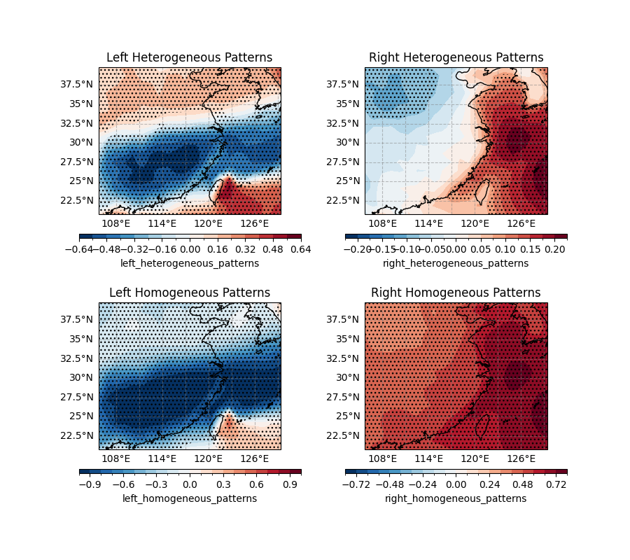
Draw the figures for both homogeneous and heterogeneous patterns
proj = ccrs.PlateCarree(central_longitude = 200)
proj_trans = ccrs.PlateCarree()

fig, ax = plt.subplots(2, 2, figsize = (9, 8), subplot_kw={"projection": proj})

# ---------------
axi = ax[0, 0]

draw_data = mca_analysis_result["heterogeneous_patterns/left_heterogeneous_patterns"].sel(mode = 2).left_heterogeneous_patterns
p_data = mca_analysis_result["heterogeneous_patterns/pvalues_of_left_heterogeneous_patterns"].sel(mode = 2).pvalues_of_left_heterogeneous_patterns

draw_data.plot.contourf(
    ax = axi, levels = 21,
    transform = proj_trans,
    cbar_kwargs={"location": "bottom", "aspect": 50, "pad" : 0.1}
)
ecl.plot.draw_significant_area_contourf(p_data, ax = axi, thresh=0.1, transform=proj_trans)

axi.coastlines()
axi.gridlines(draw_labels=["left", "bottom"], color="grey", alpha=0.5, linestyle="--")
axi.set_title('Left Heterogeneous Patterns')

# ---------------
axi = ax[0, 1]

draw_data = mca_analysis_result["heterogeneous_patterns/right_heterogeneous_patterns"].sel(mode = 2).right_heterogeneous_patterns
p_data = mca_analysis_result["heterogeneous_patterns/pvalues_of_right_heterogeneous_patterns"].sel(mode = 2).pvalues_of_right_heterogeneous_patterns

draw_data.plot.contourf(
    ax = axi, levels = 21,
    transform = proj_trans,
    cbar_kwargs={"location": "bottom", "aspect": 50, "pad" : 0.1}
)
ecl.plot.draw_significant_area_contourf(p_data, ax = axi, thresh=0.1, transform=proj_trans)

axi.coastlines()
axi.gridlines(draw_labels=["left", "bottom"], color="grey", alpha=0.5, linestyle="--")
axi.set_title('Right Heterogeneous Patterns')

# ---------------
axi = ax[1, 0]

draw_data = mca_analysis_result["homogeneous_patterns/left_homogeneous_patterns"].sel(mode = 2).left_homogeneous_patterns
p_data = mca_analysis_result["homogeneous_patterns/pvalues_of_left_homogeneous_patterns"].sel(mode = 2).pvalues_of_left_homogeneous_patterns

draw_data.plot.contourf(
    ax = axi, levels = 21,
    transform = proj_trans,
    cbar_kwargs={"location": "bottom", "aspect": 50, "pad" : 0.1}
)
ecl.plot.draw_significant_area_contourf(p_data, ax = axi, thresh=0.1, transform=proj_trans)

axi.coastlines()
axi.gridlines(draw_labels=["left", "bottom"], color="grey", alpha=0.5, linestyle="--")
axi.set_title('Left Homogeneous Patterns')

# ---------------
axi = ax[1, 1]

draw_data = mca_analysis_result["homogeneous_patterns/right_homogeneous_patterns"].sel(mode = 2).right_homogeneous_patterns
p_data = mca_analysis_result["homogeneous_patterns/pvalues_of_right_homogeneous_patterns"].sel(mode = 2).pvalues_of_right_homogeneous_patterns

draw_data.plot.contourf(
    ax = axi, levels = 21,
    vmax = 0.8, vmin = -0.8,
    cmap = "RdBu_r",
    transform = proj_trans,
    cbar_kwargs={"location": "bottom", "aspect": 50, "pad" : 0.1}
)
ecl.plot.draw_significant_area_contourf(p_data, ax = axi, thresh=0.1, transform=proj_trans)

axi.coastlines()
axi.gridlines(draw_labels=["left", "bottom"], color="grey", alpha=0.5, linestyle="--")
axi.set_title('Right Homogeneous Patterns')
Text(0.5, 1.0, 'Right Homogeneous Patterns')
Total running time of the script: (0 minutes 7.133 seconds)