Barnes Filter

Barnes filter is a commonly used spatial filtering method that mainly uses two constants g and c to calculate Gaussian weights, and performs spatial interpolation for each grid point, thus becoming a low-pass filter that filters out high-frequency fluctuations. When using two different schemes of constant g and c schemes, both retain low-frequency fluctuations of different scales. The difference between the filtering results of the two methods can result in mesoscale fluctuations.

See also

• Maddox, R. A. (1980). An Objective Technique for Separating Macroscale and Mesoscale Features in Meteorological Data. Monthly Weather Review, 108(8), 1108-1121. https://journals.ametsoc.org/view/journals/mwre/108/8/1520-0493_1980_108_1108_aotfsm_2_0_co_2.xml

• LinOuyang/pybarnes

Before proceeding with all the steps, first import some necessary libraries and packages

import matplotlib.pyplot as plt
import easyclimate as ecl

Open tuturial dataset

hgt_data = ecl.open_tutorial_dataset("hgt_2022_day5").hgt.sel(level = 500)
hgt_data

<xarray.DataArray 'hgt' (time: 5, lat: 73, lon: 144)> Size: 210kB
[52560 values with dtype=float32]
Coordinates:
  * time     (time) datetime64[ns] 40B 2022-01-01 2022-01-02 ... 2022-01-05
  * lon      (lon) float32 576B 0.0 2.5 5.0 7.5 10.0 ... 350.0 352.5 355.0 357.5
  * lat      (lat) float32 292B 90.0 87.5 85.0 82.5 ... -82.5 -85.0 -87.5 -90.0
    level    float32 4B 500.0
Attributes:
    long_name:     mean Daily Geopotential height
    units:         m
    precision:     0
    GRIB_id:       7
    GRIB_name:     HGT
    var_desc:      Geopotential height
    level_desc:    Pressure Levels
    statistic:     Mean
    parent_stat:   Individual Obs
    dataset:       NCEP Reanalysis Daily Averages
    actual_range:  [ -574.  32254.5]

xarray.DataArray

'hgt'

• time: 5
• lat: 73
• lon: 144

• ...

  [52560 values with dtype=float32]

• Coordinates: (4)
  • time
    (time)
    datetime64[ns]
    2022-01-01 ... 2022-01-05

    standard_name :

    time

    long_name :

    Time

    axis :

    T

    array(['2022-01-01T00:00:00.000000000', '2022-01-02T00:00:00.000000000',
           '2022-01-03T00:00:00.000000000', '2022-01-04T00:00:00.000000000',
           '2022-01-05T00:00:00.000000000'], dtype='datetime64[ns]')

  • lon
    (lon)
    float32
    0.0 2.5 5.0 ... 352.5 355.0 357.5

    standard_name :

    longitude

    long_name :

    Longitude

    units :

    degrees_east

    axis :

    X

    array([  0. ,   2.5,   5. ,   7.5,  10. ,  12.5,  15. ,  17.5,  20. ,  22.5,
            25. ,  27.5,  30. ,  32.5,  35. ,  37.5,  40. ,  42.5,  45. ,  47.5,
            50. ,  52.5,  55. ,  57.5,  60. ,  62.5,  65. ,  67.5,  70. ,  72.5,
            75. ,  77.5,  80. ,  82.5,  85. ,  87.5,  90. ,  92.5,  95. ,  97.5,
           100. , 102.5, 105. , 107.5, 110. , 112.5, 115. , 117.5, 120. , 122.5,
           125. , 127.5, 130. , 132.5, 135. , 137.5, 140. , 142.5, 145. , 147.5,
           150. , 152.5, 155. , 157.5, 160. , 162.5, 165. , 167.5, 170. , 172.5,
           175. , 177.5, 180. , 182.5, 185. , 187.5, 190. , 192.5, 195. , 197.5,
           200. , 202.5, 205. , 207.5, 210. , 212.5, 215. , 217.5, 220. , 222.5,
           225. , 227.5, 230. , 232.5, 235. , 237.5, 240. , 242.5, 245. , 247.5,
           250. , 252.5, 255. , 257.5, 260. , 262.5, 265. , 267.5, 270. , 272.5,
           275. , 277.5, 280. , 282.5, 285. , 287.5, 290. , 292.5, 295. , 297.5,
           300. , 302.5, 305. , 307.5, 310. , 312.5, 315. , 317.5, 320. , 322.5,
           325. , 327.5, 330. , 332.5, 335. , 337.5, 340. , 342.5, 345. , 347.5,
           350. , 352.5, 355. , 357.5], dtype=float32)

  • lat
    (lat)
    float32
    90.0 87.5 85.0 ... -87.5 -90.0

    standard_name :

    latitude

    long_name :

    Latitude

    units :

    degrees_north

    axis :

    Y

    array([ 90. ,  87.5,  85. ,  82.5,  80. ,  77.5,  75. ,  72.5,  70. ,  67.5,
            65. ,  62.5,  60. ,  57.5,  55. ,  52.5,  50. ,  47.5,  45. ,  42.5,
            40. ,  37.5,  35. ,  32.5,  30. ,  27.5,  25. ,  22.5,  20. ,  17.5,
            15. ,  12.5,  10. ,   7.5,   5. ,   2.5,   0. ,  -2.5,  -5. ,  -7.5,
           -10. , -12.5, -15. , -17.5, -20. , -22.5, -25. , -27.5, -30. , -32.5,
           -35. , -37.5, -40. , -42.5, -45. , -47.5, -50. , -52.5, -55. , -57.5,
           -60. , -62.5, -65. , -67.5, -70. , -72.5, -75. , -77.5, -80. , -82.5,
           -85. , -87.5, -90. ], dtype=float32)

  • level
    ()
    float32
    500.0

    standard_name :

    air_pressure

    long_name :

    Level

    units :

    millibar

    positive :

    down

    axis :

    Z

    actual_range :

    [1000. 10.]

    GRIB_id :

    100

    GRIB_name :

    hPa

    array(500., dtype=float32)

• Indexes: (3)
  • time
    PandasIndex

    PandasIndex(DatetimeIndex(['2022-01-01', '2022-01-02', '2022-01-03', '2022-01-04',
                   '2022-01-05'],
                  dtype='datetime64[ns]', name='time', freq=None))

  • lon
    PandasIndex

    PandasIndex(Index([  0.0,   2.5,   5.0,   7.5,  10.0,  12.5,  15.0,  17.5,  20.0,  22.5,
           ...
           335.0, 337.5, 340.0, 342.5, 345.0, 347.5, 350.0, 352.5, 355.0, 357.5],
          dtype='float32', name='lon', length=144))

  • lat
    PandasIndex

    PandasIndex(Index([ 90.0,  87.5,  85.0,  82.5,  80.0,  77.5,  75.0,  72.5,  70.0,  67.5,
            65.0,  62.5,  60.0,  57.5,  55.0,  52.5,  50.0,  47.5,  45.0,  42.5,
            40.0,  37.5,  35.0,  32.5,  30.0,  27.5,  25.0,  22.5,  20.0,  17.5,
            15.0,  12.5,  10.0,   7.5,   5.0,   2.5,   0.0,  -2.5,  -5.0,  -7.5,
           -10.0, -12.5, -15.0, -17.5, -20.0, -22.5, -25.0, -27.5, -30.0, -32.5,
           -35.0, -37.5, -40.0, -42.5, -45.0, -47.5, -50.0, -52.5, -55.0, -57.5,
           -60.0, -62.5, -65.0, -67.5, -70.0, -72.5, -75.0, -77.5, -80.0, -82.5,
           -85.0, -87.5, -90.0],
          dtype='float32', name='lat'))

• Attributes: (11)

  long_name :

  mean Daily Geopotential height

  units :

  m

  precision :

  0

  GRIB_id :

  7

  GRIB_name :

  HGT

  var_desc :

  Geopotential height

  level_desc :

  Pressure Levels

  statistic :

  Mean

  parent_stat :

  Individual Obs

  dataset :

  NCEP Reanalysis Daily Averages

  actual_range :

  [ -574. 32254.5]

Filter dataset using easyclimate.filter.calc_barnes_lowpass

hgt_data1 = ecl.filter.calc_barnes_lowpass(hgt_data)
hgt_data1

Caculating the first revision...
Caculating the second revision...

<xarray.DataArray 'hgt' (time: 5, lat: 73, lon: 144)> Size: 210kB
array([[[5222.2305, 5222.2305, 5222.2305, ..., 5235.0347, 5235.0347,
         5235.0347],
        [5200.5723, 5200.46  , 5200.3447, ..., 5190.972 , 5190.9414,
         5190.9106],
        [5174.9907, 5174.7886, 5174.5845, ..., 5154.6816, 5154.685 ,
         5154.689 ],
        ...,
        [5163.059 , 5163.5312, 5164.0054, ..., 5146.0386, 5146.181 ,
         5146.3237],
        [5128.2397, 5128.4556, 5128.676 , ..., 5115.2935, 5115.3325,
         5115.3745],
        [5097.883 , 5097.883 , 5097.883 , ..., 5083.253 , 5083.253 ,
         5083.253 ]],

       [[5263.8013, 5263.8013, 5263.8013, ..., 5278.7783, 5278.7783,
         5278.7783],
        [5236.4766, 5236.32  , 5236.162 , ..., 5232.6475, 5232.6074,
         5232.565 ],
        [5204.6294, 5204.3345, 5204.038 , ..., 5188.53  , 5188.4946,
         5188.4585],
...
        [5179.0986, 5179.465 , 5179.837 , ..., 5163.406 , 5163.4946,
         5163.586 ],
        [5156.721 , 5156.8345, 5156.951 , ..., 5147.816 , 5147.8306,
         5147.8438],
        [5143.429 , 5143.429 , 5143.429 , ..., 5145.254 , 5145.254 ,
         5145.254 ]],

       [[5000.3213, 5000.3213, 5000.3213, ..., 5003.492 , 5003.492 ,
         5003.492 ],
        [4997.3667, 4997.3325, 4997.2964, ..., 5001.8037, 5001.801 ,
         5001.796 ],
        [4997.3843, 4997.326 , 4997.266 , ..., 5004.7764, 5004.7524,
         5004.729 ],
        ...,
        [5169.53  , 5169.918 , 5170.312 , ..., 5169.401 , 5169.48  ,
         5169.563 ],
        [5137.6997, 5137.84  , 5137.9795, ..., 5134.1953, 5134.2217,
         5134.251 ],
        [5116.9644, 5116.9644, 5116.9644, ..., 5113.9883, 5113.9883,
         5113.9883]]], shape=(5, 73, 144), dtype=float32)
Coordinates:
  * time     (time) datetime64[ns] 40B 2022-01-01 2022-01-02 ... 2022-01-05
  * lon      (lon) float32 576B 0.0 2.5 5.0 7.5 10.0 ... 350.0 352.5 355.0 357.5
  * lat      (lat) float32 292B 90.0 87.5 85.0 82.5 ... -82.5 -85.0 -87.5 -90.0
    level    float32 4B 500.0

xarray.DataArray

'hgt'

• time: 5
• lat: 73
• lon: 144

• 5.222e+03 5.222e+03 5.222e+03 ... 5.114e+03 5.114e+03 5.114e+03

  array([[[5222.2305, 5222.2305, 5222.2305, ..., 5235.0347, 5235.0347,
           5235.0347],
          [5200.5723, 5200.46  , 5200.3447, ..., 5190.972 , 5190.9414,
           5190.9106],
          [5174.9907, 5174.7886, 5174.5845, ..., 5154.6816, 5154.685 ,
           5154.689 ],
          ...,
          [5163.059 , 5163.5312, 5164.0054, ..., 5146.0386, 5146.181 ,
           5146.3237],
          [5128.2397, 5128.4556, 5128.676 , ..., 5115.2935, 5115.3325,
           5115.3745],
          [5097.883 , 5097.883 , 5097.883 , ..., 5083.253 , 5083.253 ,
           5083.253 ]],
  
         [[5263.8013, 5263.8013, 5263.8013, ..., 5278.7783, 5278.7783,
           5278.7783],
          [5236.4766, 5236.32  , 5236.162 , ..., 5232.6475, 5232.6074,
           5232.565 ],
          [5204.6294, 5204.3345, 5204.038 , ..., 5188.53  , 5188.4946,
           5188.4585],
  ...
          [5179.0986, 5179.465 , 5179.837 , ..., 5163.406 , 5163.4946,
           5163.586 ],
          [5156.721 , 5156.8345, 5156.951 , ..., 5147.816 , 5147.8306,
           5147.8438],
          [5143.429 , 5143.429 , 5143.429 , ..., 5145.254 , 5145.254 ,
           5145.254 ]],
  
         [[5000.3213, 5000.3213, 5000.3213, ..., 5003.492 , 5003.492 ,
           5003.492 ],
          [4997.3667, 4997.3325, 4997.2964, ..., 5001.8037, 5001.801 ,
           5001.796 ],
          [4997.3843, 4997.326 , 4997.266 , ..., 5004.7764, 5004.7524,
           5004.729 ],
          ...,
          [5169.53  , 5169.918 , 5170.312 , ..., 5169.401 , 5169.48  ,
           5169.563 ],
          [5137.6997, 5137.84  , 5137.9795, ..., 5134.1953, 5134.2217,
           5134.251 ],
          [5116.9644, 5116.9644, 5116.9644, ..., 5113.9883, 5113.9883,
           5113.9883]]], shape=(5, 73, 144), dtype=float32)

• Coordinates: (4)
  • time
    (time)
    datetime64[ns]
    2022-01-01 ... 2022-01-05

    standard_name :

    time

    long_name :

    Time

    axis :

    T

    array(['2022-01-01T00:00:00.000000000', '2022-01-02T00:00:00.000000000',
           '2022-01-03T00:00:00.000000000', '2022-01-04T00:00:00.000000000',
           '2022-01-05T00:00:00.000000000'], dtype='datetime64[ns]')

  • lon
    (lon)
    float32
    0.0 2.5 5.0 ... 352.5 355.0 357.5

    standard_name :

    longitude

    long_name :

    Longitude

    units :

    degrees_east

    axis :

    X

    array([  0. ,   2.5,   5. ,   7.5,  10. ,  12.5,  15. ,  17.5,  20. ,  22.5,
            25. ,  27.5,  30. ,  32.5,  35. ,  37.5,  40. ,  42.5,  45. ,  47.5,
            50. ,  52.5,  55. ,  57.5,  60. ,  62.5,  65. ,  67.5,  70. ,  72.5,
            75. ,  77.5,  80. ,  82.5,  85. ,  87.5,  90. ,  92.5,  95. ,  97.5,
           100. , 102.5, 105. , 107.5, 110. , 112.5, 115. , 117.5, 120. , 122.5,
           125. , 127.5, 130. , 132.5, 135. , 137.5, 140. , 142.5, 145. , 147.5,
           150. , 152.5, 155. , 157.5, 160. , 162.5, 165. , 167.5, 170. , 172.5,
           175. , 177.5, 180. , 182.5, 185. , 187.5, 190. , 192.5, 195. , 197.5,
           200. , 202.5, 205. , 207.5, 210. , 212.5, 215. , 217.5, 220. , 222.5,
           225. , 227.5, 230. , 232.5, 235. , 237.5, 240. , 242.5, 245. , 247.5,
           250. , 252.5, 255. , 257.5, 260. , 262.5, 265. , 267.5, 270. , 272.5,
           275. , 277.5, 280. , 282.5, 285. , 287.5, 290. , 292.5, 295. , 297.5,
           300. , 302.5, 305. , 307.5, 310. , 312.5, 315. , 317.5, 320. , 322.5,
           325. , 327.5, 330. , 332.5, 335. , 337.5, 340. , 342.5, 345. , 347.5,
           350. , 352.5, 355. , 357.5], dtype=float32)

  • lat
    (lat)
    float32
    90.0 87.5 85.0 ... -87.5 -90.0

    standard_name :

    latitude

    long_name :

    Latitude

    units :

    degrees_north

    axis :

    Y

    array([ 90. ,  87.5,  85. ,  82.5,  80. ,  77.5,  75. ,  72.5,  70. ,  67.5,
            65. ,  62.5,  60. ,  57.5,  55. ,  52.5,  50. ,  47.5,  45. ,  42.5,
            40. ,  37.5,  35. ,  32.5,  30. ,  27.5,  25. ,  22.5,  20. ,  17.5,
            15. ,  12.5,  10. ,   7.5,   5. ,   2.5,   0. ,  -2.5,  -5. ,  -7.5,
           -10. , -12.5, -15. , -17.5, -20. , -22.5, -25. , -27.5, -30. , -32.5,
           -35. , -37.5, -40. , -42.5, -45. , -47.5, -50. , -52.5, -55. , -57.5,
           -60. , -62.5, -65. , -67.5, -70. , -72.5, -75. , -77.5, -80. , -82.5,
           -85. , -87.5, -90. ], dtype=float32)

  • level
    ()
    float32
    500.0

    standard_name :

    air_pressure

    long_name :

    Level

    units :

    millibar

    positive :

    down

    axis :

    Z

    actual_range :

    [1000. 10.]

    GRIB_id :

    100

    GRIB_name :

    hPa

    array(500., dtype=float32)

• Indexes: (3)
  • time
    PandasIndex

    PandasIndex(DatetimeIndex(['2022-01-01', '2022-01-02', '2022-01-03', '2022-01-04',
                   '2022-01-05'],
                  dtype='datetime64[ns]', name='time', freq=None))

  • lon
    PandasIndex

    PandasIndex(Index([  0.0,   2.5,   5.0,   7.5,  10.0,  12.5,  15.0,  17.5,  20.0,  22.5,
           ...
           335.0, 337.5, 340.0, 342.5, 345.0, 347.5, 350.0, 352.5, 355.0, 357.5],
          dtype='float32', name='lon', length=144))

  • lat
    PandasIndex

    PandasIndex(Index([ 90.0,  87.5,  85.0,  82.5,  80.0,  77.5,  75.0,  72.5,  70.0,  67.5,
            65.0,  62.5,  60.0,  57.5,  55.0,  52.5,  50.0,  47.5,  45.0,  42.5,
            40.0,  37.5,  35.0,  32.5,  30.0,  27.5,  25.0,  22.5,  20.0,  17.5,
            15.0,  12.5,  10.0,   7.5,   5.0,   2.5,   0.0,  -2.5,  -5.0,  -7.5,
           -10.0, -12.5, -15.0, -17.5, -20.0, -22.5, -25.0, -27.5, -30.0, -32.5,
           -35.0, -37.5, -40.0, -42.5, -45.0, -47.5, -50.0, -52.5, -55.0, -57.5,
           -60.0, -62.5, -65.0, -67.5, -70.0, -72.5, -75.0, -77.5, -80.0, -82.5,
           -85.0, -87.5, -90.0],
          dtype='float32', name='lat'))

• Attributes: (0)

Draw results and differences.

fig, ax = plt.subplots(3,1, figsize = (5, 15))

axi = ax[0]
hgt_data.isel(time = 0).plot.contourf(
    ax = axi, levels = 21,
    cbar_kwargs={"location": "right", "aspect": 30},
)
axi.set_title("Raw data")

axi = ax[1]
hgt_data1.isel(time = 0).plot.contourf(
    ax = axi, levels = 21,
    cbar_kwargs={"location": "right", "aspect": 30},
)
axi.set_title("Filtered data")

axi = ax[2]
draw_dta = hgt_data.isel(time = 0) - hgt_data1.isel(time = 0)
draw_dta.plot.contourf(
    ax = axi, levels = 21,
    cbar_kwargs={"location": "right", "aspect": 30},
)
axi.set_title("Mesoscale fluctuations")

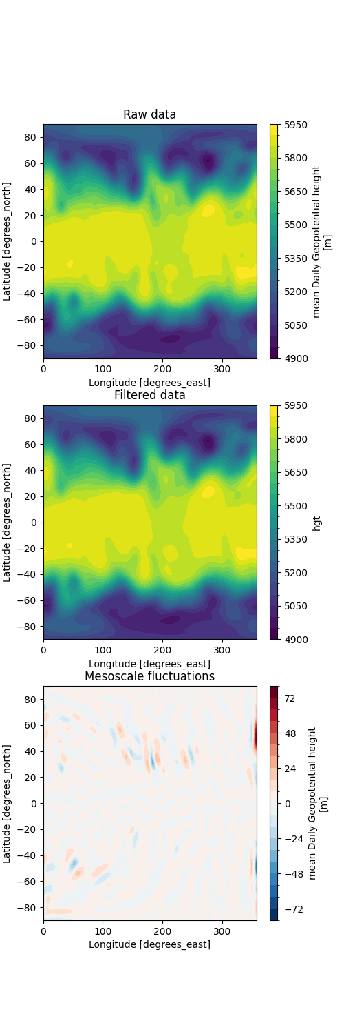
Text(0.5, 1.0, 'Mesoscale fluctuations')