Note
Go to the end to download the full example code.
Thermocline Depth and 20°C Isotherm Depth#
The ocean’s thermocline is a critical feature of the global marine environment, representing a distinct layer where water temperature decreases rapidly with depth. This transition zone separates the warm, well-mixed surface layer (typically heated by solar radiation) from the colder, denser deep ocean below. In the equatorial Pacific—an area central to global climate dynamics due to its role in phenomena like El Niño-Southern Oscillation (ENSO)—the thermocline’s depth (often referred to as the Depth of the Thermocline Core, DTC) is a key parameter. It influences heat distribution, nutrient upwelling, and air-sea interactions, making its accurate characterization essential for climate modeling and prediction.
Traditionally, the thermocline depth (DTC) is formally defined as the depth where the vertical temperature gradient \(\mathrm{d}T/\mathrm{d}z\) is maximized, denoted as \(Z_{tc}\). This definition captures the core of the thermocline, where the most significant temperature change occurs. However, directly calculating \(Z_{tc}\) requires high-resolution vertical temperature profiles, which are often sparse or computationally intensive to process. Moreover, in regions like the western Pacific warm pool—where surface waters are persistently warm and temperature gradients are relatively weak—\(Z_{tc}\) can be ambiguous or difficult to identify. These limitations have spurred the search for a simpler yet reliable proxy to represent the thermocline depth in the equatorial Pacific.
A widely adopted solution is the 20°C isotherm depth \(Z_{20}\)—the depth at which the water temperature equals 20°C. Over decades of oceanographic research, \(Z_{20}\) has emerged as a robust and practical proxy for \(Z_{tc}\) in the equatorial Pacific. Here’s why it has gained such prominence:
Proximity to the Main Thermocline Core:The 20°C isotherm lies near the center of the main thermocline in the equatorial Pacific. This region, where temperature decreases most sharply, is the thermocline’s dynamical heart. By aligning with this core, \(Z_{20}\) naturally captures the thermocline’s vertical structure, making it a physically meaningful indicator.
Consistency with :math:`Z_{tc}`: In most parts of the equatorial Pacific (excluding the warm pool), \(Z_{20}\) and \(Z_{tc}\) overlap closely. Observational data show that the depth of the 20°C isotherm closely tracks the depth of maximum vertical temperature gradient. This congruence ensures that \(Z_{20}\) reliably reflects \(Z_{tc}\) without sacrificing accuracy, even in regions where \(Z_{tc}\) might be operationally hard to define.
Practicality in Analysis: Beyond its physical relevance, \(Z_{20}\) offers practical advantages. It simplifies the study of ocean dynamics by approximating the tropical Pacific as a two-layer system: a warm upper layer above 20°C and a colder deep layer below. This approximation facilitates analysis of processes like equatorial wave propagation (e.g., Kelvin and Rossby waves) and heat transport, which are critical to ENSO variability. Additionally, \(Z_{20}\) aligns with isopycnal (constant density) surfaces, allowing researchers to link temperature structure to ocean circulation without complex 3D calculations.
Dynamical Consistency in Steady Climates: In a climate with a stable mean state (i.e., time-averaged conditions), using \(Z_{20}\) as a proxy for \(Z_{tc}\) introduces no significant dynamical inconsistency. This stability has been validated across multiple studies, confirming that \(Z_{20}\) captures the same large-scale variations in thermocline depth as \(Z_{tc}\), whether during El Niño, La Niña, or neutral conditions.
The 20°C isotherm depth \(Z_{20}\) has become a cornerstone of equatorial Pacific thermocline research. Its proximity to the thermocline core, consistency with the traditional \(Z_{tc}\) definition, analytical simplicity, and dynamical reliability make it an indispensable tool for climate scientists. By bridging the gap between theoretical definitions and practical applications, \(Z_{20}\) enhances our ability to model and predict climate variability in one of the ocean’s most climatically active regions. As ocean observing systems continue to advance, \(Z_{20}\) remains a testament to the power of finding elegant, physically grounded proxies in complex Earth system science.
See also
Yang, H., & Wang, F. (2009). Revisiting the Thermocline Depth in the Equatorial Pacific. Journal of Climate, 22(13), 3856-3863. https://doi.org/10.1175/2009JCLI2836.1
Before proceeding with all the steps, first import some necessary libraries and packages
import numpy as np
import xarray as xr
import easyclimate as ecl
import cartopy.crs as ccrs
import cartopy.feature as cfeature
import matplotlib.pyplot as plt
Preprocessed data
temper_data = xr.open_dataset('temp_soda3.4.2_mn_ocean_reg_2020_EN4.nc', chunks="auto").temp.rename({'st_ocean': 'depth'})
Warning
Here we are using only the SODA 3.4.2 reanalysis data during 2024; the actual analysis will need to be analyzed using multiple years of data.
Citation: Carton, J. A., Chepurin, G. A., & Chen, L. (2018). SODA3: A New Ocean Climate Reanalysis. Journal of Climate, 31(17), 6967-6983. https://doi.org/10.1175/JCLI-D-18-0149.1
First calculate 20°C isotherm depth (D20) through easyclimate.field.ocean.thermal.calc_D20_depth
D20_result = ecl.field.ocean.calc_D20_depth(temper_data).isel(time = 7)
D20_result.to_netcdf("sample_D20_result.nc")
Then open the dataset
D20_result = xr.open_dataarray("sample_D20_result.nc")
Then we use easyclimate.field.ocean.calc_seawater_thermocline_depth to calculate the depth of thermocline
thermocline_result = ecl.field.ocean.calc_seawater_thermocline_depth(temper_data).isel(time = 7)
thermocline_result.to_netcdf("sample_thermocline_result.nc")
Next, we open the result of thermocline
thermocline_result = xr.open_dataarray("sample_thermocline_result.nc")
Here’s the ocean thermocline depth distribution for August 2020
proj_trans = ccrs.PlateCarree()
fig, ax = ecl.plot.quick_draw_spatial_basemap(central_longitude=180)

ax.add_feature(cfeature.LAND, facecolor = '#DDDDDD', zorder = 1)

fg = thermocline_result.plot(
    vmax = 1000, vmin = 0,
    cmap = "viridis_r",
    transform = ccrs.PlateCarree(),
    add_colorbar=False,
    zorder = 0,
)
cb1 = fig.colorbar(fg, ax = ax, orientation = 'horizontal', pad = 0.15, extendrect = True)
cb1.set_label('')

ax.set_title("Thermocline (Aug., 2020)")
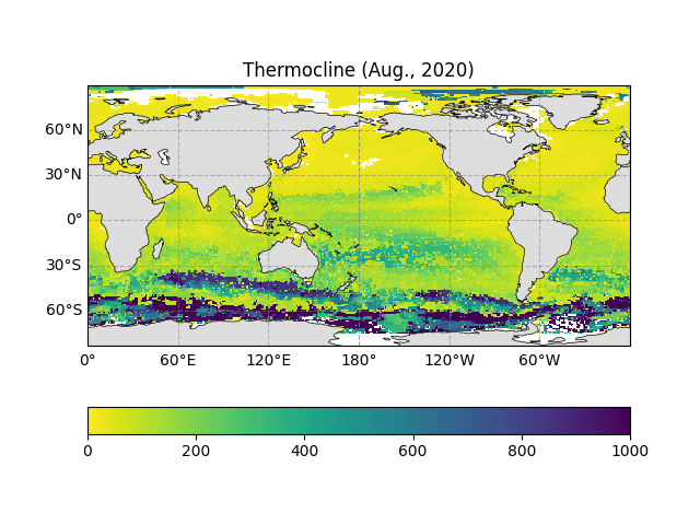
Text(0.5, 1.0, 'Thermocline (Aug., 2020)')
And the 20°C isotherm depth (D20) distribution for August 2020
proj_trans = ccrs.PlateCarree()
fig, ax = ecl.plot.quick_draw_spatial_basemap(central_longitude=180)

ax.add_feature(cfeature.LAND, facecolor = '#DDDDDD', zorder = 1)

fg = D20_result.plot(
    vmax = 1000, vmin = 0,
    cmap = "viridis_r",
    transform = ccrs.PlateCarree(),
    add_colorbar=False,
    zorder = 0,
)
cb1 = fig.colorbar(fg, ax = ax, orientation = 'horizontal', pad = 0.15, extendrect = True)
cb1.set_label('')

ax.set_title("D20 (Aug., 2020)")
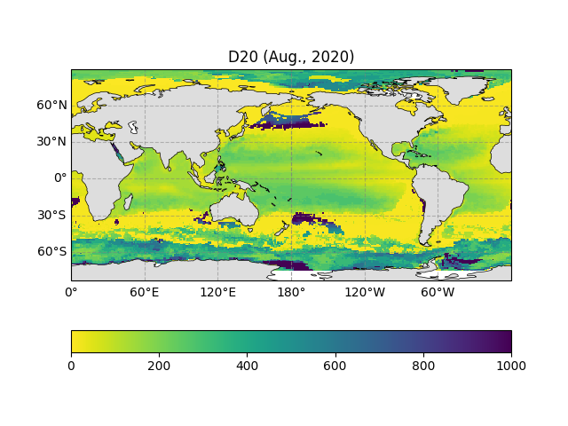
Text(0.5, 1.0, 'D20 (Aug., 2020)')
Finally we make a difference between them, and from the figure we can see that the difference is minimum in the equatorial region, meaning that in the equatorial tropics we can consider D20 to approximate the depth of the thermocline.
proj_trans = ccrs.PlateCarree()
fig, ax = ecl.plot.quick_draw_spatial_basemap(central_longitude=180)

ax.add_feature(cfeature.LAND, facecolor = '#DDDDDD', zorder = 1)

fg = (D20_result - thermocline_result).plot(
    vmax = 200,
    transform = ccrs.PlateCarree(),
    add_colorbar=False,
    zorder = 0,
)
cb1 = fig.colorbar(fg, ax = ax, orientation = 'horizontal', pad = 0.15, extendrect = True)
cb1.set_label('')

ax.set_title("Diff (Aug., 2020)")
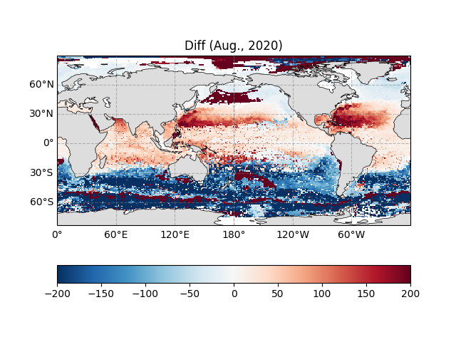
Text(0.5, 1.0, 'Diff (Aug., 2020)')
Total running time of the script: (0 minutes 3.805 seconds)