Note
Go to the end to download the full example code.
EOF Analysis of Multiple Variables#
Before proceeding with all the steps, first import some necessary libraries and packages
import xarray as xr
import matplotlib.pyplot as plt
import cartopy.crs as ccrs
import easyclimate as ecl
Load and preprocess ERA5 reanalysis data (1982-2022 850hPa wind and total precipitation),
involving vertical level selection, unit conversion (m/day to mm/day),
and Dask lazy loading for memory optimization.
u500_data = xr.open_dataset("u850_ERA5_1982-2022_N80.nc", chunks="auto").u.sel(level = 850).drop_vars("level")
v500_data = xr.open_dataset("v850_ERA5_1982-2022_N80.nc", chunks="auto").v.sel(level = 850).drop_vars("level")
tp_data = xr.open_dataset("tp_ERA5_1982-2022_N80.nc", chunks="auto").tp * 1000
Tip
You can download following datasets here:
Spatially subset data to focus on East Asia (100°E–160°E, 10°N–60°N) and sort latitude ascendingly to ensure consistent indexing and plotting.
See also
Wang, B. (1992). The Vertical Structure and Development of the ENSO Anomaly Mode during 1979–1989. Journal of Atmospheric Sciences, 49(8), 698-712. https://journals.ametsoc.org/view/journals/atsc/49/8/1520-0469_1992_049_0698_tvsado_2_0_co_2.xml
Wang, B., Wu, Z., Li, J., Liu, J., Chang, C., Ding, Y., & Wu, G. (2008). How to Measure the Strength of the East Asian Summer Monsoon. Journal of Climate, 21(17), 4449-4463. https://doi.org/10.1175/2008JCLI2183.1
Wu Bingyi, Zhang Renhe. 2011: Interannual variability of the East Asian summer monsoon and its association with the anomalous atmospheric circulation over the mid-high latitudes and external forcing. Acta Meteorologica Sinica (Chinese), (2): 219-233. http://qxxb.cmsjournal.net/article/doi/10.11676/qxxb2011.019
武炳义, 张人禾. 2011: 东亚夏季风年际变率及其与中、高纬度大气环流以及外强迫异常的联系. 气象学报, (2): 219-233. DOI: https://dx.doi.org/10.11676/qxxb2011.019
u500_data_EA = u500_data.sortby("lat").sel(lon = slice(100, 160), lat = slice(10, 60))
v500_data_EA = v500_data.sortby("lat").sel(lon = slice(100, 160), lat = slice(10, 60))
tp_data_EA = tp_data.sortby("lat").sel(lon = slice(100, 160), lat = slice(10, 60))
Initialize a multivariate EOF (MEOF) model with cosine-of-latitude weighting and seasonal cycle removal to jointly analyze wind-precipitation covariability.
model = ecl.eof.get_EOF_model(
    [u500_data_EA, v500_data_EA, tp_data_EA],
    lat_dim = 'lat', lon_dim = 'lon',
    remove_seasonal_cycle_mean = True, use_coslat = True
)
Execute EOF decomposition to compute spatial patterns, principal components, and explained variance, saving results in Zarr format for efficient persistence and reuse.
meof_analysis_result = ecl.eof.calc_EOF_analysis(model)
meof_analysis_result.to_zarr("meof_analysis_result.zarr")
Here, we load the saved dataset.
meof_analysis_result = ecl.open_datanode("./meof_analysis_result.zarr")
meof_analysis_result
Extract and downsample (every 3rd grid point) EOF spatial patterns (precipitation and winds) for the first four modes to prepare visualized data.
mode_num = 1
tp_draw_mode1 = meof_analysis_result["EOF/var2"].sel(mode = mode_num)["components"] *(-1)
u_draw = meof_analysis_result["EOF/var0"].sel(mode = mode_num)["components"]
v_draw = meof_analysis_result["EOF/var1"].sel(mode = mode_num)["components"]
uv_draw_mode1 = xr.Dataset(data_vars={"u": u_draw, "v": v_draw}).thin(lon = 3, lat = 3) *(-1)

#
mode_num = 2
tp_draw_mode2 = meof_analysis_result["EOF/var2"].sel(mode = mode_num)["components"]
u_draw = meof_analysis_result["EOF/var0"].sel(mode = mode_num)["components"]
v_draw = meof_analysis_result["EOF/var1"].sel(mode = mode_num)["components"]
uv_draw_mode2 = xr.Dataset(data_vars={"u": u_draw, "v": v_draw}).thin(lon = 3, lat = 3)

#
mode_num = 3

tp_draw_mode3 = meof_analysis_result["EOF/var2"].sel(mode = mode_num)["components"]
u_draw = meof_analysis_result["EOF/var0"].sel(mode = mode_num)["components"]
v_draw = meof_analysis_result["EOF/var1"].sel(mode = mode_num)["components"]
uv_draw_mode3 = xr.Dataset(data_vars={"u": u_draw, "v": v_draw}).thin(lon = 3, lat = 3)

#
mode_num = 4
tp_draw_mode4 = meof_analysis_result["EOF/var2"].sel(mode = mode_num)["components"]
u_draw = meof_analysis_result["EOF/var0"].sel(mode = mode_num)["components"]
v_draw = meof_analysis_result["EOF/var1"].sel(mode = mode_num)["components"]
uv_draw_mode4 = xr.Dataset(data_vars={"u": u_draw, "v": v_draw}).thin(lon = 3, lat = 3)
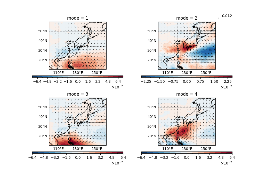
Visualize the first four MEOF modes using contourf (precipitation) and quiver (downsampled winds) on a PlateCarree projection,
with geographic context (coastlines, gridlines) for wind-precipitation covariability analysis.
proj = ccrs.PlateCarree(central_longitude = 200)
proj_trans = ccrs.PlateCarree()

fig, ax = plt.subplots(2, 2, figsize = (10, 7), subplot_kw={"projection": proj})

#
axi = ax[0, 0]
fg1 = tp_draw_mode1.plot.contourf(
    ax = axi,
    levels = 21,
    transform = proj_trans,
    add_colorbar = False
)
cb1 = fig.colorbar(fg1, ax = axi, location = 'bottom', aspect = 50, pad = 0.1, extendrect = True)
cb1.set_label('')
cb1.formatter.set_powerlimits((0, 0))
cb1.formatter.set_useMathText(True)

uv_draw_mode1.plot.quiver(
    ax = axi,
    x = "lon", y = "lat", u = "u", v = "v",
    transform = proj_trans,
)

#
axi = ax[0, 1]
fg2 = tp_draw_mode2.plot.contourf(
    ax = axi,
    levels = 21,
    transform = proj_trans,
    add_colorbar = False
)
cb2 = fig.colorbar(fg2, ax = axi, location = 'bottom', aspect = 50, pad = 0.1, extendrect = True)
cb2.set_label('')
cb2.formatter.set_powerlimits((0, 0))
cb2.formatter.set_useMathText(True)

uv_draw_mode2.plot.quiver(
    ax = axi,
    x = "lon", y = "lat", u = "u", v = "v",
    transform = proj_trans,
)

#
axi = ax[1, 0]
fg3 = tp_draw_mode3.plot.contourf(
    ax = axi,
    levels = 21,
    transform = proj_trans,
    add_colorbar = False
)
cb3 = fig.colorbar(fg3, ax = axi, location = 'bottom', aspect = 50, pad = 0.1, extendrect = True)
cb3.set_label('')
cb3.formatter.set_powerlimits((0, 0))
cb3.formatter.set_useMathText(True)

uv_draw_mode3.plot.quiver(
    ax = axi,
    x = "lon", y = "lat", u = "u", v = "v",
    transform = proj_trans,
)

#
axi = ax[1, 1]
fg4 = tp_draw_mode4.plot.contourf(
    ax = axi,
    levels = 21,
    transform = proj_trans,
    add_colorbar = False
)
cb4 = fig.colorbar(fg4, ax = axi, location = 'bottom', aspect = 50, pad = 0.1, extendrect = True)
cb4.set_label('')
cb4.formatter.set_powerlimits((0, 0))
cb4.formatter.set_useMathText(True)

uv_draw_mode4.plot.quiver(
    ax = axi,
    x = "lon", y = "lat", u = "u", v = "v",
    transform = proj_trans,
)

for axi in ax.flat:
    axi.coastlines()
    axi.gridlines(draw_labels=["left", "bottom"], color="grey", alpha=0.5, linestyle="--")
Total running time of the script: (0 minutes 2.515 seconds)