Ocean Instability

Note

Go to the end to download the full example code.

Ocean Instability#

Ocean instability refers to the tendency of the water column to undergo vertical mixing or perturbation growth due to density stratification, a critical process governing ocean dynamics, heat/salt transport, and biogeochemical cycling.

At its core, instability arises from vertical gradients in seawater density ($\rho$), primarily driven by temperature (T) and salinity (S) variations. Stable stratification (where density increases with depth) suppresses vertical motion, while unstable conditions (density decreasing with depth) promote convective overturning. Quantifying this stability is central to understanding ocean circulation, mixed layer dynamics, and climate feedbacks.

Key metrics include:

Brunt-Väisälä Frequency Squared ($N^2$): Defined as $N^2= -\frac{g}{\rho_0} \frac{\partial \rho}{\partial z}$ (where $g$ is gravitational acceleration, $\rho_0$ is reference density, and $z$ is depth), $N^2$ quantifies stratification strength. Positive $N^2$ indicates stable stratification (larger values = stronger stability), while $N^2 < 0$ signals convective instability.
Potential Density ($\rho_0$): The density of a water parcel if adiabatically brought to a reference pressure (typically surface pressure, $p=0$ dbar). It isolates density variations due to T/S from pressure effects, enabling comparison of water masses across depths.

Modern oceanographic analysis leverages TEOS-10 (Thermodynamic Equation of Seawater 2010) for accurate computation of these properties, ensuring consistency with global standards. This notebook demonstrates workflows to calculate $N^2$ and potential density from observational reanalysis data, and visualize their spatial/vertical patterns to diagnose ocean instability regimes.

See also

http://www.teos-10.org/pubs/gsw/html/gsw_Nsquared.html
http://www.teos-10.org/pubs/gsw/html/gsw_contents.html
Pawlowicz, R. (2013) Key Physical Variables in the Ocean: Temperature, Salinity, and Density. Nature Education Knowledge 4(4):13. https://www.nature.com/scitable/knowledge/library/key-physical-variables-in-the-ocean-temperature-102805293

Before proceeding with all the steps, first import some necessary libraries and packages

import numpy as np
import xarray as xr
import easyclimate as ecl
import matplotlib.pyplot as plt

Here, we import SODA 3.4.2 reanalysis data (ocean temperature and salinity) for 2020. The depth dimension "st_ocean" is renamed to "depth" for consistency, and a single time slice (time=5) is selected. These datasets serve as fundamental inputs for calculating ocean stratification metrics.

temp_data = xr.open_dataset("temp_soda3.4.2_mn_ocean_reg_2020_EN4.nc").temp.rename({"st_ocean":"depth"}).isel(time = 5)
salt_data = xr.open_dataset("salt_soda3.4.2_mn_ocean_reg_2020_EN4.nc").salt.rename({"st_ocean":"depth"}).isel(time = 5)

And we also load the mixed-layer depth data.

mld_data = xr.open_dataset("mlp_soda3.4.2_mn_ocean_reg_2020_EN4.nc").mlp.isel(time = 5)
mld_data

Tip

You can download following datasets here:

Warning

Here we are using only the SODA 3.4.2 reanalysis data during 2024.
Citation: Carton, J. A., Chepurin, G. A., & Chen, L. (2018). SODA3: A New Ocean Climate Reanalysis. Journal of Climate, 31(17), 6967-6983. https://doi.org/10.1175/JCLI-D-18-0149.1

The $N^2$ quantifies stratification stability (positive values indicate stable stratification; higher magnitudes imply stronger stability). Potential density (prho) is the density of a water parcel brought adiabatically to a reference pressure (here, surface pressure), critical for identifying water mass characteristics. Using easyclimate.field.ocean.calc_N2_from_temp_salt and easyclimate.field.ocean.calc_potential_density_from_temp_salt, these functions leverage TEOS-10 (Thermodynamic Equation of Seawater 2010) for accurate seawater property calculations. Results are saved to NetCDF files for persistent storage and downstream analysis.

N2_data = ecl.field.ocean.calc_N2_from_temp_salt(
    seawater_temperature_data = temp_data,
    seawater_practical_salinity_data = salt_data,
    time_dim = None
).N2.to_netcdf("sample_N2_data.nc")

prho_data = ecl.field.ocean.calc_potential_density_from_temp_salt(
    seawater_temperature_data = temp_data,
    seawater_practical_salinity_data = salt_data,
    time_dim = None
).prho.to_netcdf("sample_prho_data.nc")

This step verifies data integrity post-save and prepares $N^2$ for visualization/analysis. The xr.open_dataarray function ensures proper reconstruction of the labeled multi-dimensional array with metadata.

N2_data = xr.open_dataarray("sample_N2_data.nc")
N2_data

Similar to $N^2$ reloading, this step confirms successful storage and readback of potential density data, enabling subsequent spatial and vertical analysis of water mass structure.

prho_data = xr.open_dataarray("sample_prho_data.nc")
prho_data

Using easyclimate.plot.quick_draw_spatial_basemap for a pre-configured geographic basemap, the plot employs contourf to show $N^2$ magnitude, with vmax set to $5 \times 10^{-4}$ to focus on typical upper-ocean values. The colorbar is positioned at the bottom for readability. This figure highlights spatial patterns of upper-ocean stratification, with higher $N^2$ indicating stronger stability (e.g., tropical warm pools vs. mid-latitude mixed layers).

fig, ax = ecl.plot.quick_draw_spatial_basemap()

N2_data.sel(depth = slice(0, 100)).mean(dim = "depth").plot.contourf(
    vmax = 5 *10**(-4),
    levels = 21,
    cbar_kwargs = {'location': 'bottom'},
)
ax.set_title("$N^2$ (Depth Avg. from 0 to 100m)")

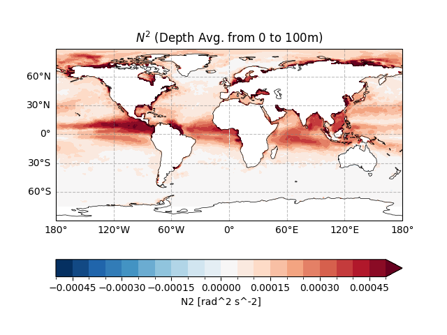
Text(0.5, 1.0, '$N^2$ (Depth Avg. from 0 to 100m)')

The plot focuses on the upper 300m to resolve the pycnocline (primary stratification layer). yincrease=False flips the y-axis to show depth increasing downward (oceanographic convention). easyclimate.plot.set_lon_format_axis formats longitude geographic labels for clarity. This visualization reveals vertical and zonal variations in stratification, such as enhanced stability in the equatorial thermocline or vertical mixing hotspots.

fig, ax = plt.subplots(figsize = (10, 4))

N2_data.sel(lat = slice(-30, 30), depth = slice(0, 300)).mean("lat").plot.contourf(
    ax = ax,
    x = 'lon', y = 'depth',
    levels = np.linspace(-8e-4, 8e-4, 21),
    yincrease = False
)

# Mixed-layer
mld_data.sel(lat = slice(-30, 30)).mean("lat").plot(color = "k")

ecl.plot.set_lon_format_axis(ax = ax)
ax.set_title("$N^2$ (Brunt-Vaisala Frequency squared)")

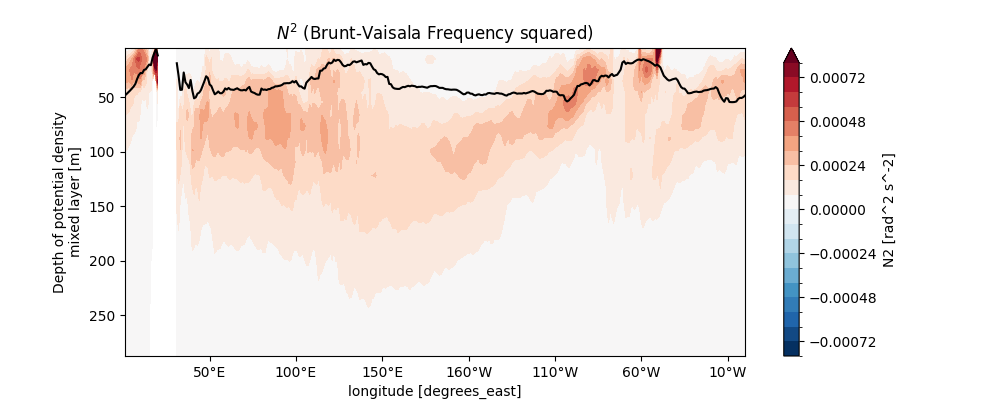
Text(0.5, 1.0, '$N^2$ (Brunt-Vaisala Frequency squared)')

Similar to the $N^2$ plot, this visualization uses contourf to display density structure, with yincrease=False for depth convention. Potential density increases with depth (due to cooling/salting), and horizontal gradients indicate geostrophic currents. Comparing with $N^2$ highlights the link between density stratification (prho vertical gradient) and stability ($N^2 \ \propto \ \frac{\partial \mathrm{prho}}{\partial z}$).

fig, ax = plt.subplots(figsize = (10, 4))

prho_data.sel(lat = slice(-30, 30), depth = slice(0, 300)).mean("lat").plot.contourf(
    ax = ax,
    x = 'lon', y = 'depth',
    levels = 21,
    yincrease = False
)

# Mixed-layer
mld_data.sel(lat = slice(-30, 30)).mean("lat").plot(color = "k")

ecl.plot.set_lon_format_axis(ax = ax)
ax.set_title("$\\rho_0$")

$\rho_0$

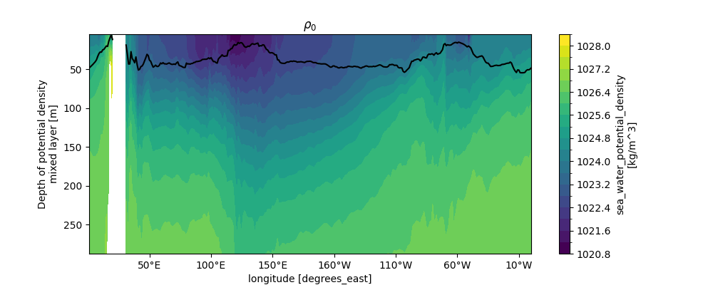
Text(0.5, 1.0, '$\\rho_0$')

Total running time of the script: (0 minutes 6.902 seconds)