Empirical Mode Decomposition (EMD) and Ensemble Empirical Mode Decomposition (EEMD)

Note

Go to the end to download the full example code.

Empirical Mode Decomposition (EMD) and Ensemble Empirical Mode Decomposition (EEMD)#

EMD (Empirical Mode Decomposition) is an adaptive time-space analysis method suitable for processing series that are non-stationary and non-linear. EMD performs operations that partition a series into ‘modes’ (IMFs; Intrinsic Mode Functions) without leaving the time domain. It can be compared to other time-space analysis methods like Fourier Transforms and wavelet decomposition. Like these methods, EMD is not based on physics. However, the modes may provide insight into various signals contained within the data. In particular, the method is useful for analyzing natural signals, which are most often non-linear and non-stationary. Some common examples would include the Southern Oscillation Index (SOI), Niño 3.4 Index, etc.

EEMD (Ensemble EMD) is a noise assisted data analysis method. EEMD consists of “sifting” an ensemble of white noise-added signal. EEMD can separate scales naturally without any a priori subjective criterion selection as in the intermittence test for the original EMD algorithm.

Wu and Huang (2009) state: “White noise is necessary to force the ensemble to exhaust all possible solutions in the sifting process, thus making the different scale signals to collate in the proper intrinsic mode functions (IMF) dictated by the dyadic filter banks. As the EMD is a time space analysis method, the white noise is averaged out with sufficient number of trials; the only persistent part that survives the averaging process is the signal, which is then treated as the true and more physical meaningful answer.” Further, they state: “EEMD represents a substantial improvement over the original EMD and is a truly noise assisted data analysis (NADA) method.”

See also

https://pyemd.readthedocs.io/
https://www.ncl.ucar.edu/Applications/eemd.shtml
https://www.clear.rice.edu/elec301/Projects02/empiricalMode/
Wu, Z., & Huang, N. E. (2009). Ensemble empirical mode decomposition: a noise-assisted data analysis method. Advances in Adaptive Data Analysis, 01(01), 1-41. https://doi.org/10.1142/S1793536909000047

Before proceeding with all the steps, first import some necessary libraries and packages

import xarray as xr
import matplotlib.pyplot as plt
import easyclimate as ecl

Load and inspect Niño 3 SST anomaly data The dataset contains monthly sea surface temperature anomalies in the Niño 3 region, a key indicator for ENSO monitoring and analysis

data = xr.open_dataset("test_input_nino3_wavelet.nc")["nino3"]
data

<xarray.DataArray 'nino3' (time: 504)> Size: 4kB
[504 values with dtype=float64]
Coordinates:
  * time     (time) datetime64[ns] 4kB 1871-01-31 1871-04-30 ... 1996-10-31

Perform Empirical Mode Decomposition (EMD) on the time series EMD decomposes the nonlinear, non-stationary signal into intrinsic mode functions (IMFs) representing oscillatory modes embedded in the data at different timescales The time_step=”M” parameter indicates monthly resolution of the input data

imf_result = ecl.filter.filter_emd(data, time_step="M")
imf_result

Perform Ensemble Empirical Mode Decomposition (EEMD) on the time series EEMD improves upon EMD by adding white noise ensembles to overcome mode mixing The method performs multiple EMD trials (default=100) with different noise realizations and averages the results to obtain more stable IMF components

eimf_result = ecl.filter.filter_eemd(data, time_step="M")
eimf_result

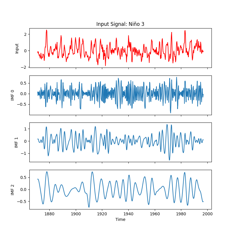
Visualize the first three IMF components from standard EMD IMFs are ordered from highest frequency (IMF0) to lowest frequency (IMF2) Each IMF must satisfy two conditions:

Number of extrema and zero crossings differs by at most one
Mean of upper and lower envelopes is zero at any point

fig, ax = plt.subplots(4, 1, figsize = (8, 8), sharex=True)
fig.subplots_adjust(hspace=0.2)

axi = ax[0]
imf_result["input"].plot(ax = axi, color = "r")
axi.set_xlabel("")
axi.set_ylabel("Input")
axi.set_title("Input Signal: Niño 3")

axi = ax[1]
imf_result["imf0"].plot(ax = axi)
axi.set_xlabel("")
axi.set_ylabel("IMF 0")

axi = ax[2]
imf_result["imf1"].plot(ax = axi)
axi.set_xlabel("")
axi.set_ylabel("IMF 1")

axi = ax[3]
imf_result["imf2"].plot(ax = axi)
axi.set_xlabel("Time")
axi.set_ylabel("IMF 2")

Text(51.222222222222214, 0.5, 'IMF 2')

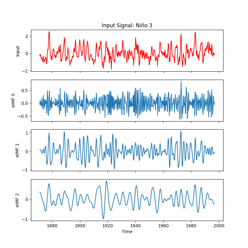
Visualize the first three eIMF components from EEMD Ensemble IMFs show improved mode separation compared to standard EMD The noise-assisted approach helps distinguish:

High-frequency noise/oscillations (eIMF0)
Seasonal-to-interannual variability (eIMF1)
Lower frequency trends (eIMF2)

fig, ax = plt.subplots(4, 1, figsize = (8, 8), sharex=True)
fig.subplots_adjust(hspace=0.2)

axi = ax[0]
eimf_result["input"].plot(ax = axi, color = "r")
axi.set_xlabel("")
axi.set_ylabel("Input")
axi.set_title("Input Signal: Niño 3")

axi = ax[1]
eimf_result["eimf0"].plot(ax = axi)
axi.set_xlabel("")
axi.set_ylabel("eIMF 0")

axi = ax[2]
eimf_result["eimf1"].plot(ax = axi)
axi.set_xlabel("")
axi.set_ylabel("eIMF 1")

axi = ax[3]
eimf_result["eimf2"].plot(ax = axi)
axi.set_xlabel("Time")
axi.set_ylabel("eIMF 2")

Text(64.22222222222221, 0.5, 'eIMF 2')

Total running time of the script: (0 minutes 6.407 seconds)