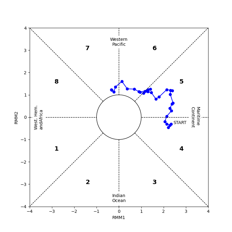
MJO Phase Space Trajectory Diagram

Before proceeding with all the steps, first import some necessary libraries and packages

import xarray as xr
import pandas as pd
import easyclimate as ecl
import matplotlib.pyplot as plt

Load MJO phase space data

mjo_ds = xr.open_dataset('http://iridl.ldeo.columbia.edu/SOURCES/.BoM/.MJO/.RMM/dods',
                         decode_times=False)
T = mjo_ds.T.values
mjo_ds['T'] = pd.date_range("1974-06-01", periods=len(T))
mjo_ds = ecl.utility.get_compress_xarraydata(mjo_ds)
mjo_ds.to_netcdf("mjo_data.nc")

Modify the name of the time parameter

Tip

You can download following datasets here: Download mjo_data.nc

mjo_data = xr.open_dataset("mjo_data.nc").rename({"T": "time"})
mjo_data

<xarray.Dataset> Size: 446kB
Dimensions:    (time: 18566)
Coordinates:
  * time       (time) datetime64[ns] 149kB 1974-06-01 1974-06-02 ... 2025-03-30
Data variables:
    amplitude  (time) float32 74kB ...
    phase      (time) float32 74kB ...
    RMM1       (time) float32 74kB ...
    RMM2       (time) float32 74kB ...

xarray.Dataset

• Dimensions:
  • time: 18566
• Coordinates: (1)
  • time
    (time)
    datetime64[ns]
    1974-06-01 ... 2025-03-30

    array(['1974-06-01T00:00:00.000000000', '1974-06-02T00:00:00.000000000',
           '1974-06-03T00:00:00.000000000', ..., '2025-03-28T00:00:00.000000000',
           '2025-03-29T00:00:00.000000000', '2025-03-30T00:00:00.000000000'],
          shape=(18566,), dtype='datetime64[ns]')

• Data variables: (4)
  • amplitude
    (time)
    float32
    ...

    [18566 values with dtype=float32]

  • phase
    (time)
    float32
    ...

    [18566 values with dtype=float32]

  • RMM1
    (time)
    float32
    ...

    [18566 values with dtype=float32]

  • RMM2
    (time)
    float32
    ...

    [18566 values with dtype=float32]

• Indexes: (1)
  • time
    PandasIndex

    PandasIndex(DatetimeIndex(['1974-06-01', '1974-06-02', '1974-06-03', '1974-06-04',
                   '1974-06-05', '1974-06-06', '1974-06-07', '1974-06-08',
                   '1974-06-09', '1974-06-10',
                   ...
                   '2025-03-21', '2025-03-22', '2025-03-23', '2025-03-24',
                   '2025-03-25', '2025-03-26', '2025-03-27', '2025-03-28',
                   '2025-03-29', '2025-03-30'],
                  dtype='datetime64[ns]', name='time', length=18566, freq=None))

• Attributes: (0)

Draw MJO Phase Space Trajectory Diagram

fig, ax = plt.subplots(figsize = (7.5, 7.5))

ecl.field.equatorial_wave.draw_mjo_phase_space_basemap()
ecl.field.equatorial_wave.draw_mjo_phase_space(
    mjo_data = mjo_data.sel(time = slice('2024-12-01', '2024-12-31')),
    rmm1_dim = "RMM1",
    rmm2_dim = "RMM2",
    time_dim = "time"
)