
Note
Go to the end to download the full example code.
Water Flux Divergence
This example shows how to calculate water vapor flux divergence on pressure levels and for the vertically integrated water vapor flux. Positive values indicate horizontal water vapor flux divergence, while negative values indicate horizontal convergence.
Before proceeding with all the steps, first import some necessary libraries and packages
import easyclimate as ecl
import xarray as xr
import numpy as np
import matplotlib.pyplot as plt
import cartopy.crs as ccrs
import matplotlib.ticker as mticker
Read sample data
The calculation uses pressure-level wind and specific humidity fields. Surface pressure is required for the column-integrated water vapor flux divergence.
u_data = ecl.open_tutorial_dataset("uwnd_2022_day5")["uwnd"].sortby("lat")
v_data = ecl.open_tutorial_dataset("vwnd_2022_day5")["vwnd"].sortby("lat")
q_data = ecl.open_tutorial_dataset("shum_2022_day5")["shum"].sortby("lat")
slp_data = ecl.open_tutorial_dataset("pres_2022_day5")["pres"].sortby("lat")
Configure scientific notation for the contour-plot colorbars.
import matplotlib.ticker as ticker
formatter = ticker.ScalarFormatter(useMathText=True, useOffset=True)
formatter.set_powerlimits((0, 0))
Define a reusable map background so each plot uses the same geographic domain, coastlines, and gridline labels.
def draw_base_background(ax, lonlat_range):
    ax.set_extent(lonlat_range, crs=ccrs.PlateCarree())
    ax.coastlines(resolution="50m", linewidth=0.8, color="grey")
    gl = ax.gridlines(
        crs=ccrs.PlateCarree(),
        draw_labels=True,
        linewidth=0.5,
        color="gray",
        alpha=0.4,
        linestyle="--"
    )
    gl.top_labels = False
    gl.right_labels = False
    gl.left_labels = True
    gl.bottom_labels = True
    gl.xlocator = mticker.FixedLocator([80, 100, 120, 140, 160, 180])
    gl.ylocator = mticker.FixedLocator([0, 10, 20, 30, 40, 50, 60, 70])
Single-Level Water Vapor Flux Divergence
easyclimate.calc_divergence_watervaporflux
calculates water vapor flux divergence at each pressure level:
The Rust backend is the default high-performance method and is recommended for normal use.
qflux_div_rs = ecl.calc_divergence_watervaporflux(
    specific_humidity_data = q_data,
    qu_data = u_data,
    qv_data = v_data,
    specific_humidity_data_units = "kg/kg",
    # The following parameters generally do not need to be passed
    method = "rust-batch",
)
qflux_div_rs
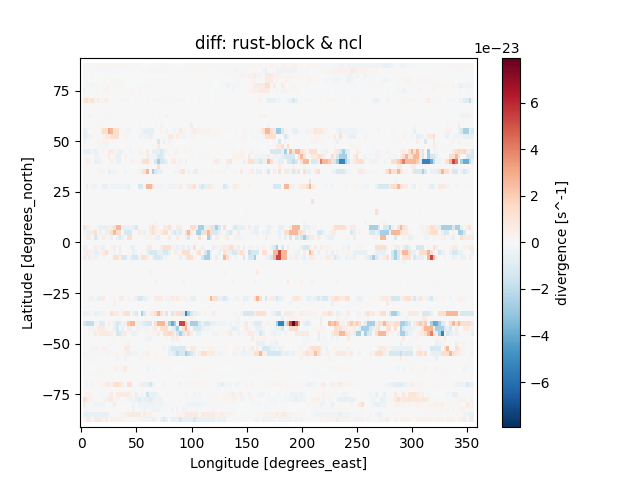
For numerical comparison, calculate the same field with the NCL-compatible backend and plot the difference against the Rust result.
qflux_div_ncl = ecl.calc_divergence_watervaporflux(
    specific_humidity_data = q_data,
    qu_data = u_data,
    qv_data = v_data,
    specific_humidity_data_units = "kg/kg",
    # The following parameters generally do not need to be passed
    method = "ncl",
)

diff_qflux_div = qflux_div_rs - qflux_div_ncl
diff_qflux_div.sel(level = 850).isel(time = 2).plot()
plt.title("diff: rust-block & ncl")
Text(0.5, 1.0, 'diff: rust-block & ncl')
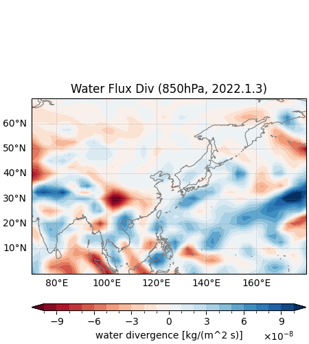
Plot the water vapor flux divergence at 850 hPa on 2022-01-03. Negative values correspond to moisture-flux convergence, while positive values correspond to moisture-flux divergence.
lonlat_range = [70, 180, 0, 70]

fig, ax = plt.subplots(
    1, 1,
    figsize=(4.5, 5),
    subplot_kw={"projection": ccrs.PlateCarree()},
    constrained_layout=True
)

draw_base_background(ax, lonlat_range)

qflux_div_rs.sel(level = 850).isel(time = 2).plot.contourf(
    ax = ax,
    transform=ccrs.PlateCarree(),
    levels = np.linspace(-1e-7, 1e-7, 21),
    cmap = "RdBu",
    cbar_kwargs = {'location': 'bottom', 'aspect': 40, 'format': formatter, 'label': "water divergence [kg/(m^2 s)]"},
)

ax.set_title("Water Flux Div (850hPa, 2022.1.3)")
Text(0.5, 1.0, 'Water Flux Div (850hPa, 2022.1.3)')
Vertically Integrated Water Vapor Flux Divergence
easyclimate.calc_divergence_watervaporflux_top2surface_integral
first integrates water vapor flux through the atmospheric column and then
calculates its horizontal divergence:
The vertical coordinate is level in hPa, while the surface pressure field
is supplied in Pa.
qflux_div_integral_rs = ecl.calc_divergence_watervaporflux_top2surface_integral(
    specific_humidity_data = q_data,
    u_data = u_data,
    v_data = v_data,
    surface_pressure_data = slp_data,
    vertical_dim = "level",
    specific_humidity_data_units = "kg/kg",
    surface_pressure_data_units = "Pa",
    vertical_dim_units = "hPa",
    # The following parameters generally do not need to be passed
    integral_method = "rust-block", # default
    div_method = "rust-batch", # default
)
qflux_div_integral_rs
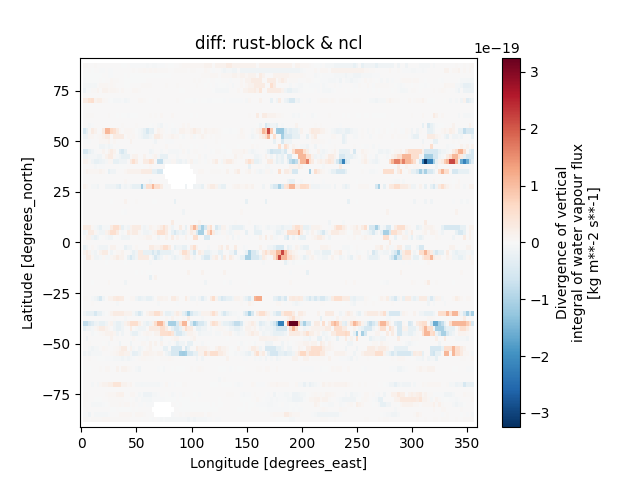
Repeat the column-integrated calculation with the NCL-compatible integration and divergence methods. This block is intended for numerical testing rather than routine analysis.
qflux_div_integral_ncl = ecl.calc_divergence_watervaporflux_top2surface_integral(
    specific_humidity_data = q_data,
    u_data = u_data,
    v_data = v_data,
    surface_pressure_data = slp_data,
    vertical_dim = "level",
    specific_humidity_data_units = "kg/kg",
    surface_pressure_data_units = "Pa",
    vertical_dim_units = "hPa",
    # For numerical tests only
    integral_method = "ncl",
    div_method = "ncl",
)

diff_qflux_div_integral = qflux_div_integral_rs - qflux_div_integral_ncl
diff_qflux_div_integral.isel(time = 2)["wvdiv"].plot()
plt.title("diff: rust-block & ncl")
Text(0.5, 1.0, 'diff: rust-block & ncl')
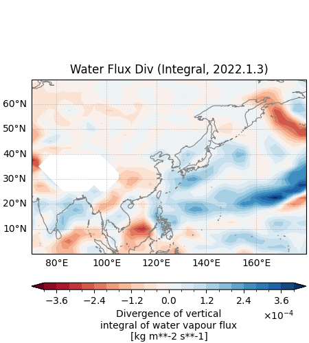
Plot the vertically integrated water vapor flux divergence. This field is commonly used to diagnose column moisture convergence and divergence.
lonlat_range = [70, 180, 0, 70]


fig, ax = plt.subplots(
    1, 1,
    figsize=(4.5, 5),
    subplot_kw={"projection": ccrs.PlateCarree()},
    constrained_layout=True
)

draw_base_background(ax, lonlat_range)

qflux_div_integral_rs["wvdiv"].isel(time = 2).plot.contourf(
    ax = ax,
    transform=ccrs.PlateCarree(),
    levels = np.linspace(-4e-4, 4e-4, 21),
    cmap = "RdBu",
    cbar_kwargs = {'location': 'bottom', 'aspect': 40, 'format': formatter},
)

ax.set_title("Water Flux Div (Integral, 2022.1.3)")
Text(0.5, 1.0, 'Water Flux Div (Integral, 2022.1.3)')
Total running time of the script: (0 minutes 17.751 seconds)