Maximum Eady Growth Rate

Note

Go to the end to download the full example code.

Maximum Eady Growth Rate#

Think of the atmosphere as a giant, swirling dance of air masses. Sometimes these dances become unstable and form dramatic weather systems like storms and cyclones. The Eady Growth Rate is like a “storm predictor” - it tells us how quickly these weather systems can grow and intensify!

Technically speaking, the Eady Growth Rate measures how fast weather disturbances can amplify in a rotating, stratified atmosphere. It was first derived from the famous Eady model in 1949 and has become a fundamental tool for meteorologists ever since.

The mathematical formula looks like this:

\[\sigma = 0.3098 \frac{f}{N} \frac{\mathrm{d} U}{\mathrm{d} z}\]

Where:

$\sigma$ is the Eady growth rate (how fast storms grow)
$f$ is the Coriolis parameter (Earth’s rotation effect)
$N$ is the Brunt-Väisälä frequency (atmosphere’s stability)
$\frac{\mathrm{d} U}{\mathrm{d} z}$ is the vertical wind shear (how wind changes with height)

Caution

The Eady growth rate is a non-linear quantity, so you should NOT apply it directly to monthly averaged data. If you want monthly EGR values, calculate EGR first using daily data, then compute the monthly average!

See also

Eady, E. T. (1949). Long Waves and Cyclone Waves. Tellus, 1(3), 33–52. https://doi.org/10.3402/tellusa.v1i3.8507, https://www.tandfonline.com/doi/abs/10.3402/tellusa.v1i3.8507
Lindzen, R. S. , & Farrell, B. (1980). A Simple Approximate Result for the Maximum Growth Rate of Baroclinic Instabilities. Journal of Atmospheric Sciences, 37(7), 1648-1654. https://journals.ametsoc.org/view/journals/atsc/37/7/1520-0469_1980_037_1648_asarft_2_0_co_2.xml
Simmonds, I., and E.-P. Lim (2009), Biases in the calculation of Southern Hemisphere mean baroclinic eddy growth rate, Geophys. Res. Lett., 36, L01707, https://doi.org/10.1029/2008GL036320.
Sloyan, B. M., and T. J. O’Kane (2015), Drivers of decadal variability in the Tasman Sea, J. Geophys. Res. Oceans, 120, 3193–3210, https://doi.org/10.1002/2014JC010550.
eady_growth_rate -NCL

First, we import our tools! Think of this as gathering our weather forecasting equipment, and also set up a special number formatter to make our scientific notation look clean and professional!

import easyclimate as ecl
import cartopy.crs as ccrs
import cmaps
import matplotlib.ticker as ticker

formatter = ticker.ScalarFormatter(useMathText=True, useOffset=True)
formatter.set_powerlimits((0, 0))

Time to load our weather ingredients! We’re gathering three key ingredients:

Zonal Wind (uwnd_daily): The east-west component of wind - imagine the wind blowing from west to east
Geopotential Height (z_daily): Think of this as the “height” of pressure levels in the atmosphere
Temperature (temp_daily): The air temperature at different levels

Attention

The geopotential height data should be meters, NOT $\mathrm{m^2 \cdot s^2}$ which is the unit used in the representation of potential energy.

We use sortby("lat") to ensure our latitude data is properly organized from south to north.

uwnd_daily = (
    ecl.open_tutorial_dataset("uwnd_2022_day5")
    .uwnd.sortby("lat")
)
z_daily = (
    ecl.open_tutorial_dataset("hgt_2022_day5")
    .hgt.sortby("lat")
)
temp_daily = (
    ecl.open_tutorial_dataset("air_2022_day5")
    .air.sortby("lat")
)

uwnd_2022_day5.nc ━━━━━━━━━━━━━━━━━━━━ 100.0% • 2.2/2.2 MB • 69.7 MB/s • 0:00:00
hgt_2022_day5.nc ━━━━━━━━━━━━━━━━━━━━━ 100.0% • 1.7/1.7 MB • 62.5 MB/s • 0:00:00
air_2022_day5.nc ━━━━━━━━━━━━━━━━━━━━━ 100.0% • 1.9/1.9 MB • 75.1 MB/s • 0:00:00

Now for the magic! 🎩 We call the easyclimate.calc_eady_growth_rate function with our three weather ingredients:

vertical_dim="level" tells the function that our vertical coordinate is called “level”
vertical_dim_units="hPa" specifies that we’re using hectopascals (the standard unit for atmospheric pressure levels)

The function returns a treasure trove of information:

eady_growth_rate: Our main star - the maximum Eady growth rate.
dudz: The vertical wind shear.
brunt_vaisala_frequency: The Brunt-Väisälä frequency (atmospheric stability).

We use .isel(time=3) to select the fourth time step (Python counts from 0!) for visualization.

egr_result = ecl.calc_eady_growth_rate(
    u_daily_data=uwnd_daily,
    z_daily_data=z_daily,
    temper_daily_data=temp_daily,
    vertical_dim="level",
    vertical_dim_units="hPa",
).isel(time=3)
egr_result

/opt/hostedtoolcache/Python/3.11.14/x64/lib/python3.11/site-packages/xarray/computation/apply_ufunc.py:818: RuntimeWarning: invalid value encountered in sqrt
  result_data = func(*input_data)

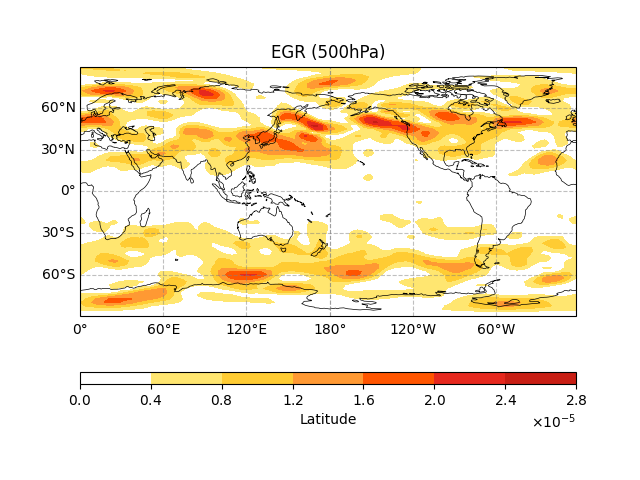
Time to see our results! We create a world map and plot the Eady Growth Rate at 500 hPa (about 5.5 km altitude).

The red and yellow areas show where storms are most likely to grow rapidly - these are the “storm nurseries” of the atmosphere! The color scale uses scientific notation (like $1.2 \cdot 10^{-5}$) to handle the very small numbers typical in atmospheric physics.

fig, ax = ecl.plot.quick_draw_spatial_basemap(central_longitude=180)

egr_result.eady_growth_rate.sel(level = 500).plot.contourf(
    ax = ax,
    transform = ccrs.PlateCarree(),
    cbar_kwargs = {'location': 'bottom', 'aspect': 40, 'format': formatter},
    cmap = cmaps.sunshine_9lev
)
ax.set_title("EGR (500hPa)")

Text(0.5, 1.0, 'EGR (500hPa)')

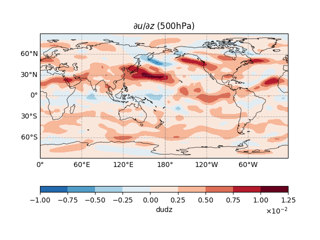
This plot shows the vertical wind shear - how much the wind speed changes as you go higher in the atmosphere.

Think of it like this: if you’re in an elevator and the wind is much stronger at the top floor than the ground floor, that’s strong vertical shear! This shear provides the “fuel” for storm development.

fig, ax = ecl.plot.quick_draw_spatial_basemap(central_longitude=180)

egr_result.dudz.sel(level = 500).plot.contourf(
    ax = ax,
    transform = ccrs.PlateCarree(),
    cbar_kwargs = {'location': 'bottom', 'aspect': 40, 'format': formatter}
)
ax.set_title("$\\partial u / \\partial z$ (500hPa)")

$$\partial u / \partial z$ (500hPa)$

Text(0.5, 1.0, '$\\partial u / \\partial z$ (500hPa)')

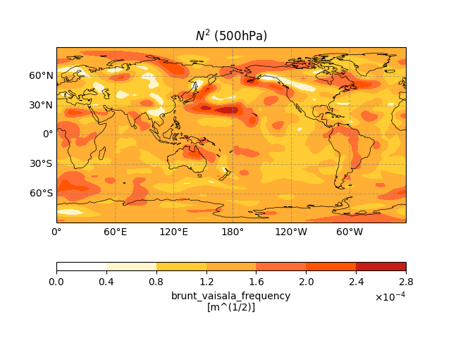
Finally, we plot the Brunt-Väisälä frequency squared ($N^2$), which measures how stable the atmosphere is.

High values mean the atmosphere is very stable (like a well-behaved layer cake), while low values indicate instability (like a wobbly jelly). Storms love unstable atmospheres because it’s easier for air parcels to rise and form clouds!

fig, ax = ecl.plot.quick_draw_spatial_basemap(central_longitude=180)

(egr_result.brunt_vaisala_frequency **2).sel(level = 500).plot.contourf(
    ax = ax,
    transform = ccrs.PlateCarree(),
    cbar_kwargs = {'location': 'bottom', 'aspect': 40, 'format': formatter},
    cmap = cmaps.sunshine_9lev
)
ax.set_title("$N^2$ (500hPa)")

Text(0.5, 1.0, '$N^2$ (500hPa)')

Total running time of the script: (0 minutes 3.689 seconds)