Note
Go to the end to download the full example code.
Wave Activity Horizontal Flux
Rossby waves are like giant atmospheric ripples that guide the movement of weather systems across the midlatitudes. When these waves amplify or propagate downstream, they can help explain why blocking highs, troughs, and persistent cold or warm events appear in preferred regions.
Wave activity flux (WAF) offers a compact way to diagnose both the strength and the direction of that propagation. In practice, the flux vectors behave a bit like arrows showing where stationary wave energy is traveling.
This example demonstrates two commonly used horizontal WAF diagnostics:
easyclimate.calc_TN_wave_activity_horizontal_fluxfor the Takaya and Nakamura (2001) formulation, which includes the effect of a background climatological flow.easyclimate.calc_Plumb_wave_activity_horizontal_fluxfor the Plumb (1985) formulation, which is widely used for stationary planetary waves.
In all examples below, the geopotential height anomaly must be provided in meters, not in \(\mathrm{m^2\ s^{-2}}\).
See also
Plumb, R. A., 1985: On the Three-Dimensional Propagation of Stationary Waves. J. Atmos. Sci., 42, 217–229. https://journals.ametsoc.org/view/journals/atsc/42/3/1520-0469_1985_042_0217_ottdpo_2_0_co_2.xml
Takaya, K., & Nakamura, H. (2001). A Formulation of a Phase-Independent Wave-Activity Flux for Stationary and Migratory Quasigeostrophic Eddies on a Zonally Varying Basic Flow. Journal of the Atmospheric Sciences, 58(6), 608-627. https://journals.ametsoc.org/view/journals/atsc/58/6/1520-0469_2001_058_0608_afoapi_2.0.co_2.xml
First, import the plotting and analysis packages. We also configure a scientific-notation formatter so the colorbar labels remain clean when plotting large or small atmospheric quantities.
import easyclimate as ecl
import cartopy.crs as ccrs
import cmaps
import matplotlib.pyplot as plt
import matplotlib.ticker as ticker
import numpy as np

formatter = ticker.ScalarFormatter(useMathText=True, useOffset=True)
formatter.set_powerlimits((0, 0))
Next, load the anomaly field and the climatological basic-state winds.
z500_prime_data1andz500_prime_data2are 500 hPa geopotential height anomalies for two different Novembers.u500_climatology_dataandv500_climatology_dataprovide the monthly climatological background flow required by the TN01 formulation.We divide geopotential height by
9.8so the anomaly is expressed in meters.
Sorting by latitude keeps the map grids ordered from south to north before plotting.
z500_prime_data1 = ecl.open_tutorial_dataset("era5_daily_z500_prime_201411_N15.nc").z /9.8
z500_prime_data2 = ecl.open_tutorial_dataset("era5_daily_z500_prime_202411_N15.nc").z /9.8
u500_climatology_data = ecl.open_tutorial_dataset("era5_ymean_monthly_u500_199101_202012_N15.nc").u.sortby("lat")
v500_climatology_data = ecl.open_tutorial_dataset("era5_ymean_monthly_v500_199101_202012_N15.nc").v.sortby("lat")
z500_prime_data1 = z500_prime_data1.sortby("lat")
z500_prime_data2 = z500_prime_data2.sortby("lat")
era5_daily_z500_prime_201411_N15.nc ━━━━━━━ 100.0% • 229.2/… • 11.2    • 0:00:00
                                                     kB        MB/s
era5_daily_z500_prime_202411_N15.nc ━━━━━━━ 100.0% • 227.9/… • 14.7    • 0:00:00
                                                     kB        MB/s
era5_ymean_monthly_u500_199101_202012_N15.nc ━━━━ 100.0% • 125.… • 11.0 • 0:00:…
                                                           kB      MB/s
era5_ymean_monthly_v500_199101_202012_N15.nc ━━━━ 100.0% • 126.… • 6.1  • 0:00:…
                                                           kB      MB/s
TN01 Wave Activity Horizontal Flux
We start with the Takaya-Nakamura horizontal wave activity flux.
The function easyclimate.calc_TN_wave_activity_horizontal_flux returns an xarray.Dataset containing:
psi_p: perturbation streamfunction,fx: zonal component of the flux,fy: meridional component of the flux.
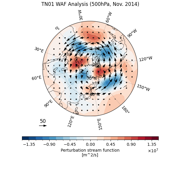
Here we diagnose the November 2014 case and then average over time to obtain the monthly-mean propagation pattern.
tn01_result1 = ecl.calc_TN_wave_activity_horizontal_flux(
    z_prime_data = z500_prime_data1,
    u_climatology_data = u500_climatology_data,
    v_climatology_data = v500_climatology_data,
    vertical_dim = "level",
    vertical_dim_units = "hPa",
)
tn01_result1
tn01_mean_result1 = tn01_result1.mean(dim = "time").sortby("lat")
tn01_mean_result1
To make a continuous global contour map, we add a cyclic longitude point to the scalar field. The vector field is kept on the original grid and will be thinned during plotting.
draw_shaded1 = tn01_mean_result1["psi_p"]
draw_shaded1 = ecl.plot.add_lon_cyclic(draw_shaded1, 6)
draw_quiver1 = tn01_mean_result1[["fx", "fy"]]
This first figure uses a polar stereographic projection, which is especially helpful for viewing Rossby-wave trains across the Northern Hemisphere.
Shading shows the perturbation streamfunction, while the arrows show the horizontal WAF vectors. Larger arrows indicate stronger downstream propagation of wave activity.
fig, ax = plt.subplots(
    figsize = (6, 6),
    subplot_kw={"projection": ccrs.NorthPolarStereo(central_longitude=140)}
)

ax.coastlines(color="black", linewidths=0.5)
gl, meta = ecl.plot.draw_polar_basemap(
    ax = ax,
    lon_step=30,
    lat_step=20,
    lat_range=[10, 90],
    draw_labels=True,
    gridlines_kwargs={"color": "grey", "alpha": 0.5, "linestyle": "--"},
    lat_label_lon=-60
)

fg1 = draw_shaded1.plot.contourf(
    ax = ax,
    levels = np.linspace(-1.5e7, 1.5e7, 21),
    cbar_kwargs = {'location': 'bottom', 'aspect': 40, 'format': formatter},
    transform=ccrs.PlateCarree(),
    cmap = "RdBu_r",
    zorder = 1,
)

q = draw_quiver1.sel(lat = slice(10, None)).plot.quiver(
    ax = ax,
    x = "lon", y = "lat", u = "fx", v = "fy",
    transform = ccrs.PlateCarree(),
    scale = 600,
    regrid_shape = 18,
    headwidth = 5,
    width = 0.0045,
    headlength = 8,
    headaxislength = 8,
    minlength = 3,
    add_guide = False,
    zorder = 2,
)
qk = ax.quiverkey(
    q, 0, -0.1,
    50, "50", labelpos = "N",
    color = "k",
    coordinates = "axes",
    fontproperties = {"size": 12},
    labelsep = 0.05,
    transform = ccrs.PlateCarree(),
)
qk.set_zorder(3)

ax.set_title("")
ecl.plot.set_polar_title("TN01 WAF Analysis (500hPa, Nov. 2014)", meta, size = 15)
Text(0.5, 1.0864137921696746, 'TN01 WAF Analysis (500hPa, Nov. 2014)')
The same calculation can be repeated for a different year. Because the TN01 scheme automatically matches each time step to the corresponding climatological month, it is convenient for composite and event analyses.
tn01_result2 = ecl.calc_TN_wave_activity_horizontal_flux(
    z_prime_data = z500_prime_data2,
    u_climatology_data = u500_climatology_data,
    v_climatology_data = v500_climatology_data,
    vertical_dim = "level",
    vertical_dim_units = "hPa",
)
tn01_mean_result2 = tn01_result2.mean(dim = "time").sortby("lat")
tn01_mean_result2
draw_shaded2 = tn01_mean_result2["psi_p"]
draw_shaded2 = ecl.plot.add_lon_cyclic(draw_shaded2, 6)
draw_quiver2 = tn01_mean_result2[["fx", "fy"]]
This second TN01 map uses a Mercator projection to emphasize the downstream extension of the wave train over Eurasia and the North Pacific.
fig, ax = plt.subplots(
    figsize = (12, 6),
    subplot_kw={"projection": ccrs.Mercator(central_longitude=140)}
)
ax.set_extent([0, 360, 10, 85], crs = ccrs.PlateCarree())
ax.coastlines(color="black", linewidths=0.5)
ax.gridlines(draw_labels=["bottom", "left"], alpha=0)

fg1 = draw_shaded2.plot.contourf(
    ax = ax,
    levels = np.linspace(-1e7, 1e7, 21),
    cbar_kwargs = {'location': 'bottom', 'aspect': 80, 'shrink': 0.7, 'pad': 0.1, 'format': formatter},
    transform=ccrs.PlateCarree(),
    cmap = "RdBu_r",
    zorder = 1,
)

q = draw_quiver2.sel(lat = slice(5, None)).plot.quiver(
    ax = ax,
    x = "lon", y = "lat", u = "fx", v = "fy",
    transform = ccrs.PlateCarree(),
    scale = 800,
    regrid_shape = 15,
    add_guide = False,
)
qk = ax.quiverkey(
    q, 0.95, 1.03,
    50, "50", labelpos = "N",
    color = "k",
    coordinates = "axes",
    fontproperties = {"size": 12},
    labelsep = 0.05,
    transform = ccrs.PlateCarree(),
)

ax.set_title("TN01 WAF Analysis (500hPa, Nov. 2024)")

Text(0.5, 1.0, 'TN01 WAF Analysis (500hPa, Nov. 2024)')
Plumb Wave Activity Horizontal Flux
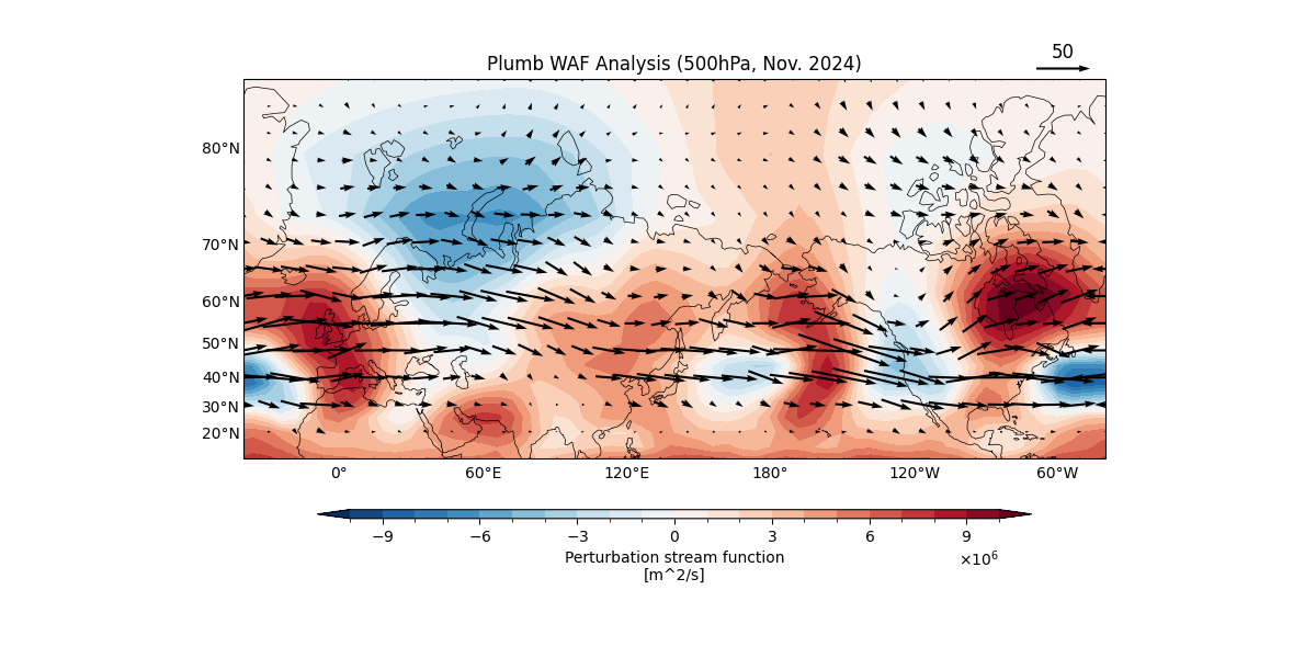
Now switch to the Plumb horizontal flux.
easyclimate.calc_Plumb_wave_activity_horizontal_flux uses only the geopotential height anomaly field and is especially suitable for diagnosing stationary wave propagation.
pwaf_result = ecl.calc_Plumb_wave_activity_horizontal_flux(
    z_prime_data = z500_prime_data2,
    vertical_dim = "level",
    vertical_dim_units = "hPa",
)
pwaf_mean_result = pwaf_result.mean(dim = "time").sortby("lat")
pwaf_mean_result
draw_shaded3 = pwaf_mean_result["psi_p"]
draw_shaded3 = ecl.plot.add_lon_cyclic(draw_shaded3, 6)
draw_quiver3 = pwaf_mean_result[["fx", "fy"]]
The plotting procedure is identical, which makes comparison between the TN01 and Plumb diagnostics straightforward.
If the two flux patterns are broadly similar, that often indicates a robust stationary Rossby-wave signal. Differences can reflect the role of the background climatological flow included in the TN01 formulation.
fig, ax = plt.subplots(
    figsize = (12, 6),
    subplot_kw={"projection": ccrs.Mercator(central_longitude=140)}
)
ax.set_extent([0, 360, 10, 85], crs = ccrs.PlateCarree())
ax.coastlines(color="black", linewidths=0.5)
ax.gridlines(draw_labels=["bottom", "left"], alpha=0)

fg1 = draw_shaded3.plot.contourf(
    ax = ax,
    levels = np.linspace(-1e7, 1e7, 21),
    cbar_kwargs = {'location': 'bottom', 'aspect': 80, 'shrink': 0.7, 'pad': 0.1, 'format': formatter},
    transform=ccrs.PlateCarree(),
    cmap = "RdBu_r",
    zorder = 1,
)

q = draw_quiver3.sel(lat = slice(5, None)).plot.quiver(
    ax = ax,
    x = "lon", y = "lat", u = "fx", v = "fy",
    transform = ccrs.PlateCarree(),
    scale = 800,
    regrid_shape = 15,
    add_guide = False,
)
qk = ax.quiverkey(
    q, 0.95, 1.03,
    50, "50", labelpos = "N",
    color = "k",
    coordinates = "axes",
    fontproperties = {"size": 12},
    labelsep = 0.05,
    transform = ccrs.PlateCarree(),
)

ax.set_title("Plumb WAF Analysis (500hPa, Nov. 2024)")
Text(0.5, 1.0, 'Plumb WAF Analysis (500hPa, Nov. 2024)')
These figures provide a compact visual summary of wave propagation:
Shading highlights the perturbation streamfunction pattern associated with the geopotential height anomaly.
Vectors indicate the direction and relative strength of downstream wave activity propagation.
TN01 flux is generally preferred when a spatially varying background flow is important.
Plumb flux is a classic diagnostic for large-scale stationary Rossby waves.
Total running time of the script: (0 minutes 6.603 seconds)