Note
Go to the end to download the full example code.
Geographic Finite Difference
Before proceeding with all the steps, first import some necessary libraries and packages
import easyclimate as ecl
import xarray as xr
import matplotlib.pyplot as plt
import cartopy.crs as ccrs
Then consider obtaining meridional and zonal wind variables in tutorial data
Tip
You can download following datasets here:
u_data = ecl.tutorial.open_tutorial_dataset("uwnd_202201_mon_mean").sortby("lat").uwnd
v_data = ecl.tutorial.open_tutorial_dataset("vwnd_202201_mon_mean").sortby("lat").vwnd
z_data = ecl.tutorial.open_tutorial_dataset("hgt_202201_mon_mean").sortby("lat").hgt
temp_data = ecl.tutorial.open_tutorial_dataset("air_202201_mon_mean").sortby("lat").air
q_data = ecl.tutorial.open_tutorial_dataset("shum_202201_mon_mean").sortby("lat").shum
msl_data = (
    ecl.tutorial.open_tutorial_dataset("pressfc_202201_mon_mean").sortby("lat").pres
)
pr_data = (
    ecl.tutorial.open_tutorial_dataset("precip_202201_mon_mean").sortby("lat").precip
)

uvdata = xr.Dataset()
uvdata["uwnd"] = u_data
uvdata["vwnd"] = v_data
vwnd_202201_mon_mean.nc ━━━━━━━━━━━━━━ 100.0% • 1.2/1.2 MB • 28.4 MB/s • 0:00:00
hgt_202201_mon_mean.nc ━━━━━━━━━━━━ 100.0% • 960.5/960.5   • 24.1 MB/s • 0:00:00
                                             kB
air_202201_mon_mean.nc ━━━━━━━━━━━━━━━ 100.0% • 1.1/1.1 MB • 33.6 MB/s • 0:00:00
shum_202201_mon_mean.nc ━━━━━━━━━━━━ 100.0% • 603.3/603.3  • 17.0 MB/s • 0:00:00
                                              kB
pressfc_202201_mon_mean.nc ━━━━━━━━━━━ 100.0% • 98.7/98.7   • 4.3 MB/s • 0:00:00
                                                kB
precip_202201_mon_mean.nc ━━━━━━━━━━━━ 100.0% • 74.4/74.4   • 4.7 MB/s • 0:00:00
                                                kB
Obtain data slices on 500hPa isobars for January 2022
uvdata_500_202201 = uvdata.sel(level=500, time="2022-01-01")
z_data_500_202201 = z_data.sel(level=500, time="2022-01-01")
temp_data_500_202201 = temp_data.sel(level=500, time="2022-01-01")
Plotting a sample quiver plot of this data slice
fig, ax = plt.subplots(
    subplot_kw={"projection": ccrs.PlateCarree(central_longitude=180)}
)

ax.stock_img()
ax.gridlines(draw_labels=["bottom", "left"], color="grey", alpha=0.5, linestyle="--")
ax.coastlines(edgecolor="black", linewidths=0.5)

uvdata_500_202201.thin(lon=3, lat=3).plot.quiver(
    ax=ax,
    u="uwnd",
    v="vwnd",
    x="lon",
    y="lat",
    # projection on data
    transform=ccrs.PlateCarree(),
)
![time = 2022-01-01, level = 500.0 [millibar]](../../_images/sphx_glr_plot_geographic_finite_difference_001.png)
<matplotlib.quiver.Quiver object at 0x7f1a756fd390>
First-order Partial Derivative
Consider the function easyclimate.calc_gradient to compute the gradient of the zonal wind with respect to longitude.
The argument dim to the function easyclimate.calc_gradient specifies that the direction of the solution is longitude.
uwnd_dx = ecl.calc_gradient(uvdata_500_202201.uwnd, dim="lon")

uwnd_dx
fig, ax = plt.subplots(
    subplot_kw={"projection": ccrs.PlateCarree(central_longitude=180)}
)

ax.stock_img()
ax.gridlines(draw_labels=["bottom", "left"], color="grey", alpha=0.5, linestyle="--")
ax.coastlines(edgecolor="black", linewidths=0.5)

uwnd_dx.plot.contourf(
    ax=ax,
    # projection on data
    transform=ccrs.PlateCarree(),
    # Colorbar is placed at the bottom
    cbar_kwargs={"location": "bottom"},
    levels=21,
)
![time = 2022-01-01, level = 500.0 [millibar]](../../_images/sphx_glr_plot_geographic_finite_difference_002.png)
<cartopy.mpl.contour.GeoContourSet object at 0x7f1a74fe1b90>
Of course, it is also possible to pass in xarray.Dataset directly into the function easyclimate.calc_gradient to iterate through all the variables, so that you can get the gradient of both the zonal and meridional winds with respect to longitude at the same time.
uvwnd_dx = ecl.calc_gradient(uvdata_500_202201, dim="lon")

uvwnd_dx
However, if one is required to solve for the gradient of the zonal wind with respect to the corresponding distance at each longitude, the function calc_dx_gradient should be used to calculate.
uwnd_dlon = ecl.calc_dx_gradient(uvdata_500_202201.uwnd, lon_dim="lon", lat_dim="lat")

fig, ax = plt.subplots(
    subplot_kw={"projection": ccrs.PlateCarree(central_longitude=180)}
)

ax.gridlines(draw_labels=["bottom", "left"], color="grey", alpha=0.5, linestyle="--")
ax.coastlines(edgecolor="black", linewidths=0.5)

uwnd_dlon.plot.contourf(
    ax=ax,
    # projection on data
    transform=ccrs.PlateCarree(),
    # Colorbar is placed at the bottom
    cbar_kwargs={"location": "bottom"},
    levels=21,
)
![time = 2022-01-01, level = 500.0 [millibar]](../../_images/sphx_glr_plot_geographic_finite_difference_003.png)
<cartopy.mpl.contour.GeoContourSet object at 0x7f1a750c7e10>
Similarly, use easyclimate.calc_dy_gradient to solve for the gradient of the meridional wind with respect to the corresponding distance at each latitude.
Second-order Partial Derivative
The solution of the second-order partial derivative relies on three functional calculations
easyclimate.calc_dx_laplacian: calculation of the second-order partial derivative term (Laplace term) along longitude.
uwnd_dlon2 = ecl.calc_dx_laplacian(
    uvdata_500_202201.uwnd, lon_dim="lon", lat_dim="lat"
)
easyclimate.calc_dy_laplacian: calculation of the second-order partial derivative term (Laplace term) along latitude.
uwnd_dlat2 = ecl.calc_dy_laplacian(uvdata_500_202201.uwnd, lat_dim="lat")
easyclimate.calc_dxdy_mixed_derivatives: second-order mixed partial derivative terms along longitude and latitude.
uwnd_dlonlat = ecl.calc_dxdy_mixed_derivatives(
    uvdata_500_202201.uwnd, lon_dim="lon", lat_dim="lat"
)
Second-order partial derivative term along longitude.
fig, ax = plt.subplots(
    subplot_kw={"projection": ccrs.PlateCarree(central_longitude=180)}
)

ax.gridlines(draw_labels=["bottom", "left"], color="grey", alpha=0.5, linestyle="--")
ax.coastlines(edgecolor="black", linewidths=0.5)

uwnd_dlon2.plot.contourf(
    ax=ax, transform=ccrs.PlateCarree(), cbar_kwargs={"location": "bottom"}, levels=21
)
ax.set_title("$\\frac{\\partial^2 F}{\\partial x^2}$", fontsize=20)
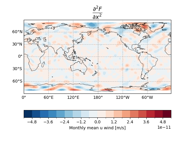
Text(0.5, 1.0326797365031362, '$\\frac{\\partial^2 F}{\\partial x^2}$')
Second-order partial derivative term along latitude.
fig, ax = plt.subplots(
    subplot_kw={"projection": ccrs.PlateCarree(central_longitude=180)}
)

ax.gridlines(draw_labels=["bottom", "left"], color="grey", alpha=0.5, linestyle="--")
ax.coastlines(edgecolor="black", linewidths=0.5)

uwnd_dlat2.plot.contourf(
    ax=ax, transform=ccrs.PlateCarree(), cbar_kwargs={"location": "bottom"}, levels=21
)
ax.set_title("$\\frac{\\partial^2 F}{\\partial y^2}$", fontsize=20)
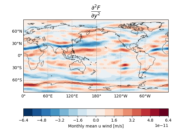
Text(0.5, 1.0480710965501792, '$\\frac{\\partial^2 F}{\\partial y^2}$')
Second-order mixed partial derivative terms along longitude and latitude.
fig, ax = plt.subplots(
    subplot_kw={"projection": ccrs.PlateCarree(central_longitude=180)}
)

ax.gridlines(draw_labels=["bottom", "left"], color="grey", alpha=0.5, linestyle="--")
ax.coastlines(edgecolor="black", linewidths=0.5)

uwnd_dlonlat.plot.contourf(
    ax=ax, transform=ccrs.PlateCarree(), cbar_kwargs={"location": "bottom"}, levels=21
)
ax.set_title("$\\frac{\\partial^2 F}{\\partial x \\partial y}$", fontsize=20)
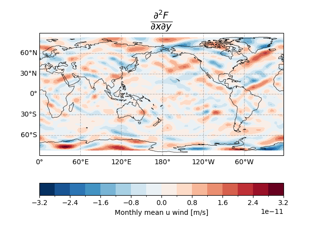
Text(0.5, 1.02873053875448, '$\\frac{\\partial^2 F}{\\partial x \\partial y}$')
Vorticity and Divergence
Vorticity and divergence are measures of the degree of atmospheric rotation and volumetric flux per unit volume respectively. For vorticity and divergence in the quasi-geostrophic case, the potential height is used as input data for the calculations. In general, we first calculate the quasi-geostrophic wind.
easyclimate.calc_geostrophic_wind: calculate the geostrophic wind.
geostrophic_wind_data_500_202201 = ecl.calc_geostrophic_wind(
    z_data_500_202201, lon_dim="lon", lat_dim="lat"
)
The function easyclimate.calc_vorticity is then used to compute the quasi-geostrophic vorticity.
easyclimate.calc_vorticity: calculate the horizontal relative vorticity term.
qg_vor_data_500_202201 = ecl.calc_vorticity(
    u_data=geostrophic_wind_data_500_202201.ug,
    v_data=geostrophic_wind_data_500_202201.vg,
    lon_dim="lon",
    lat_dim="lat",
)

qg_vor_data_500_202201.sel(lat=slice(20, 80)).plot.contourf(levels=21)
![time = 2022-01-01, level = 500.0 [millibar]](../../_images/sphx_glr_plot_geographic_finite_difference_007.png)
<matplotlib.contour.QuadContourSet object at 0x7f1a74fe9b90>
Similar vorticity for actual winds, but for actual winds rather than quasi-geostrophic winds.
vor_data_500_202201 = ecl.calc_vorticity(
    u_data=uvdata_500_202201["uwnd"],
    v_data=uvdata_500_202201["vwnd"],
    lon_dim="lon",
    lat_dim="lat",
)

vor_data_500_202201.sel(lat=slice(20, 80)).plot.contourf(levels=21)
![time = 2022-01-01, level = 500.0 [millibar]](../../_images/sphx_glr_plot_geographic_finite_difference_008.png)
<matplotlib.contour.QuadContourSet object at 0x7f1a746eadd0>
In addition, the function easyclimate.calc_divergence calculate the quasi-geostrophic divergence.
easyclimate.calc_divergence: calculate the horizontal divergence term.
Quasi-geostrophic divergence
qg_div_data_500_202201 = ecl.calc_divergence(
    u_data=geostrophic_wind_data_500_202201.ug,
    v_data=geostrophic_wind_data_500_202201.vg,
    lon_dim="lon",
    lat_dim="lat",
)

qg_div_data_500_202201.sel(lat=slice(20, 80)).plot.contourf(levels=21)
![time = 2022-01-01, level = 500.0 [millibar]](../../_images/sphx_glr_plot_geographic_finite_difference_009.png)
<matplotlib.contour.QuadContourSet object at 0x7f1a7474a610>
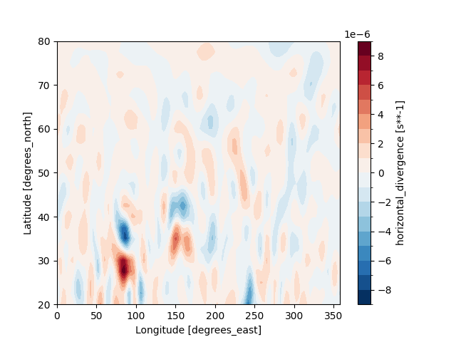
Actual divergence
div_data_500_202201 = ecl.calc_divergence(
    u_data=uvdata_500_202201["uwnd"],
    v_data=uvdata_500_202201["vwnd"],
    lon_dim="lon",
    lat_dim="lat",
)

div_data_500_202201.sel(lat=slice(20, 80)).plot.contourf(levels=21)
![time = 2022-01-01, level = 500.0 [millibar]](../../_images/sphx_glr_plot_geographic_finite_difference_010.png)
<matplotlib.contour.QuadContourSet object at 0x7f1a7462a610>
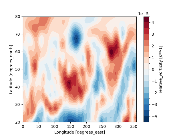
Of course, in addition to the built-in finite difference method, the spherical harmonic function mothod can be solved, but you must ensure that it is Global and Regular or Gaussian grid type data.
easyclimate.windspharm.calc_relative_vorticity: calculate the relative vorticity term with the spherical harmonic function mothod.easyclimate.windspharm.calc_divergence: calculate the horizontal divergence term with the spherical harmonic function mothod.
vor_data_500_202201_windspharm = ecl.windspharm.calc_relative_vorticity(
    u_data=uvdata_500_202201["uwnd"],
    v_data=uvdata_500_202201["vwnd"],
)

vor_data_500_202201_windspharm.sortby("lat").sel(lat=slice(20, 80)).plot.contourf(
    levels=21
)
<matplotlib.contour.QuadContourSet object at 0x7f1a74591c90>
div_data_500_202201_windspharm = ecl.windspharm.calc_divergence(
    u_data=uvdata_500_202201["uwnd"],
    v_data=uvdata_500_202201["vwnd"],
)

div_data_500_202201_windspharm.sortby("lat").sel(lat=slice(20, 80)).plot.contourf(
    levels=21
)
<matplotlib.contour.QuadContourSet object at 0x7f1a74442610>
Generally speaking, the calculation results of the finite difference method and the spherical harmonic function method are similar. The former does not require global regional data, but the calculation results of the latter are more accurate for high latitude regions.
Advection
Advection is the process of transport of an atmospheric property solely by the mass motion (velocity field) of the atmosphere; also, the rate of change of the value of the advected property at a given point.
For zonal advection, we can calculate as follows.
u_advection_500_202201 = ecl.calc_u_advection(
    u_data=uvdata_500_202201["uwnd"], temper_data=temp_data_500_202201
)

u_advection_500_202201.sortby("lat").sel(lat=slice(20, 80)).plot.contourf(levels=21)
![time = 2022-01-01, level = 500.0 [millibar]](../../_images/sphx_glr_plot_geographic_finite_difference_013.png)
<matplotlib.contour.QuadContourSet object at 0x7f1a74339b90>
Similarly, the meridional advection can acquire as follows.
v_advection_500_202201 = ecl.calc_v_advection(
    v_data=uvdata_500_202201["vwnd"], temper_data=temp_data_500_202201
)

v_advection_500_202201.sortby("lat").sel(lat=slice(20, 80)).plot.contourf(levels=21)
![time = 2022-01-01, level = 500.0 [millibar]](../../_images/sphx_glr_plot_geographic_finite_difference_014.png)
<matplotlib.contour.QuadContourSet object at 0x7f1a74209a90>
Water Flux
easyclimate.calc_horizontal_water_flux: calculate horizontal water vapor flux at each vertical level.
easyclimate.calc_vertical_water_flux: calculate vertical water vapor flux.
easyclimate.calc_water_flux_top2surface_integral: calculate the water vapor flux across the vertical level.
easyclimate.calc_horizontal_water_flux can calculate the horizontal water flux of single layers.
ecl.calc_horizontal_water_flux(
    specific_humidity_data=q_data,
    u_data=uvdata.uwnd,
    v_data=uvdata.vwnd,
)
The whole layer integral needs to consider the function easyclimate.calc_water_flux_top2surface_integral to calculate.
water_flux_top2surface_integral = ecl.calc_water_flux_top2surface_integral(
    specific_humidity_data=q_data,
    u_data=u_data,
    v_data=v_data,
    surface_pressure_data=msl_data,
    surface_pressure_data_units="millibars",
    specific_humidity_data_units = "kg/kg",
    vertical_dim="level",
    vertical_dim_units="hPa",
)

water_flux_top2surface_integral
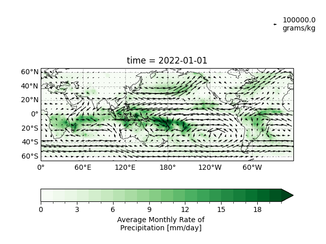
Extracting the entire layer water vapor flux at mid and low latitudes at the 0th time level.
draw_water_flux = (
    water_flux_top2surface_integral.isel(time=0)
    .thin(lon=3, lat=3)
    .sel(lat=slice(-60, 60))
)
draw_pr = pr_data.isel(time=0).sel(lat=slice(-60, 60))
fig, ax = plt.subplots(
    subplot_kw={"projection": ccrs.PlateCarree(central_longitude=180)}
)

ax.gridlines(draw_labels=["bottom", "left"], color="grey", alpha=0.5, linestyle="--")
ax.coastlines(edgecolor="black", linewidths=0.5)

draw_water_flux.plot.quiver(
    ax=ax,
    u="qu",
    v="qv",
    x="lon",
    y="lat",
    transform=ccrs.PlateCarree(),
    zorder=2,
)

draw_pr.plot.contourf(
    ax=ax,
    transform=ccrs.PlateCarree(),
    levels=21,
    cmap="Greens",
    zorder=1,
    cbar_kwargs={"location": "bottom"},
    vmax=20,
)
<cartopy.mpl.contour.GeoContourSet object at 0x7f1a7476ad50>
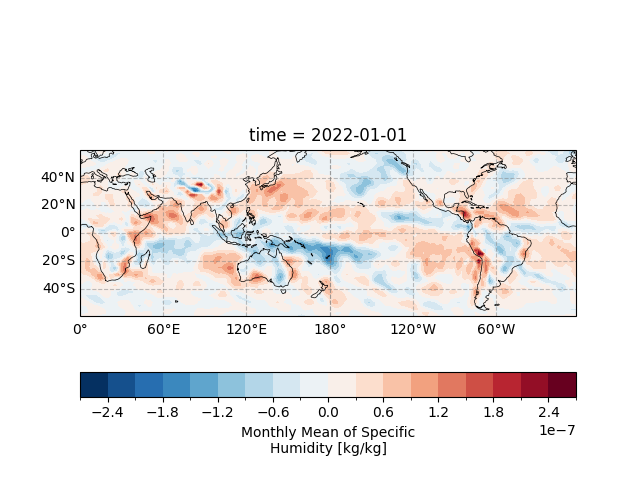
Water Vapor Flux Divergence
Water vapor flux divergence represents the convergence and divergence of water vapor. There are also two built-in functions to calculate the results of single-layers and whole-layer integration respectively.
easyclimate.calc_divergence_watervaporflux: calculate water vapor flux divergence at each vertical level.
easyclimate.calc_divergence_watervaporflux_top2surface_integral: calculate water vapor flux divergence across the vertical level.
divergence_watervaporflux_top2surface_integral = (
    ecl.calc_divergence_watervaporflux_top2surface_integral(
        specific_humidity_data=q_data,
        u_data=u_data,
        v_data=v_data,
        surface_pressure_data=msl_data,
        surface_pressure_data_units="millibars",
        specific_humidity_data_units="grams/kg",
        vertical_dim="level",
        vertical_dim_units="hPa",
    )
)

divergence_watervaporflux_top2surface_integral
Extracting the entire layer water vapor flux at mid and low latitudes at the 0th time level.
draw_data = divergence_watervaporflux_top2surface_integral.isel(time=0).sel(
    lat=slice(-60, 60)
).wvdiv
fig, ax = plt.subplots(
    subplot_kw={"projection": ccrs.PlateCarree(central_longitude=180)}
)

ax.gridlines(draw_labels=["bottom", "left"], color="grey", alpha=0.5, linestyle="--")
ax.coastlines(edgecolor="black", linewidths=0.5)

draw_data.plot.contourf(
    ax=ax, transform=ccrs.PlateCarree(), cbar_kwargs={"location": "bottom"}, levels=21
)
<cartopy.mpl.contour.GeoContourSet object at 0x7f1a751197d0>
Total running time of the script: (0 minutes 23.646 seconds)