
Note
Go to the end to download the full example code.
Water Flux
This example shows how to calculate horizontal water vapor flux on pressure levels and its vertical integral from the top of the atmosphere to the surface. The input fields are specific humidity, zonal wind, meridional wind, and surface pressure.
Before proceeding with all the steps, first import some necessary libraries and packages
import easyclimate as ecl
import xarray as xr
import numpy as np
import matplotlib.pyplot as plt
import cartopy.crs as ccrs
import matplotlib.ticker as mticker
Read sample data
The wind and specific humidity fields are pressure-level data. The surface pressure field is used when integrating the flux through the atmospheric column.
u_data = ecl.open_tutorial_dataset("uwnd_2022_day5")["uwnd"].sortby("lat")
v_data = ecl.open_tutorial_dataset("vwnd_2022_day5")["vwnd"].sortby("lat")
q_data = ecl.open_tutorial_dataset("shum_2022_day5")["shum"].sortby("lat")
slp_data = ecl.open_tutorial_dataset("pres_2022_day5")["pres"].sortby("lat")
uwnd_2022_day5.nc ━━━━━━━━━━━━━━━━━━━━ 100.0% • 2.2/2.2 MB • 53.1 MB/s • 0:00:00
vwnd_2022_day5.nc ━━━━━━━━━━━━━━━━━━━━ 100.0% • 2.2/2.2 MB • 43.3 MB/s • 0:00:00
shum_2022_day5.nc ━━━━━━━━━━━━━━━━━━━━ 100.0% • 1.2/1.2 MB • 33.6 MB/s • 0:00:00
pres_2022_day5.nc ━━━━━━━━━━━━━━━━━ 100.0% • 122.6/122.6 kB • 5.1 MB/s • 0:00:00
Define a small helper for the map background. Keeping this in a function makes the single-level and vertically integrated plots use the same map extent, coastlines, and grid labels.
def draw_base_background(ax, lonlat_range):
    ax.set_extent(lonlat_range, crs=ccrs.PlateCarree())
    ax.coastlines(resolution="50m", linewidth=0.8, color="grey")
    gl = ax.gridlines(
        crs=ccrs.PlateCarree(),
        draw_labels=True,
        linewidth=0.5,
        color="gray",
        alpha=0.4,
        linestyle="--"
    )
    gl.top_labels = False
    gl.right_labels = False
    gl.left_labels = True
    gl.bottom_labels = True
    gl.xlocator = mticker.FixedLocator([80, 100, 120, 140, 160, 180])
    gl.ylocator = mticker.FixedLocator([0, 10, 20, 30, 40, 50, 60, 70])
Horizontal Water Vapor Flux
easyclimate.calc_horizontal_water_flux
calculates water vapor flux at each pressure level:
The result is an xarray.Dataset with two
components:
qu: zonal water vapor fluxqv: meridional water vapor flux
Plot the horizontal water vapor flux at 850 hPa on 2022-01-03. The vectors show the direction and relative magnitude of water vapor transport.
lonlat_range = [70, 180, 0, 70]

fig, ax = plt.subplots(
    1, 1,
    figsize=(4.5, 5),
    subplot_kw={"projection": ccrs.PlateCarree()},
    constrained_layout=True
)

draw_base_background(ax, lonlat_range)

qflux.isel(time = 2).sel(level = 850).plot.quiver(
    x = "lon", y = "lat", u = "qu", v = "qv",
    transform=ccrs.PlateCarree(),
    regrid_shape = 15,
    scale = 0.1,
    add_guide = False
)

ax.set_title("Water Flux (850hPa, 2022.1.3)")
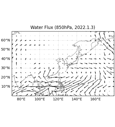
Text(0.5, 1.0, 'Water Flux (850hPa, 2022.1.3)')
Vertically Integrated Water Vapor Flux
easyclimate.calc_water_flux_top2surface_integral
integrates the horizontal water vapor flux over the atmospheric column:
The pressure coordinate is given by vertical_dim="level" and
vertical_dim_units="hPa". Since the surface pressure field is in Pa, set
surface_pressure_data_units="Pa" explicitly.
qflux_integral = ecl.calc_water_flux_top2surface_integral(
    specific_humidity_data = q_data,
    u_data = u_data,
    v_data = v_data,
    surface_pressure_data = slp_data,
    vertical_dim = "level",
    specific_humidity_data_units = "kg/kg",
    surface_pressure_data_units = "Pa",
    vertical_dim_units = "hPa",
    # support backend method selection, e.g., "ncl", "rust", "rust-batch"
    # The following parameters generally do not need to be passed
    method = "rust-block"
)
qflux_integral
Plot the vertically integrated flux. Compared with the single-level result, this vector field represents the column-integrated horizontal moisture transport.
lonlat_range = [70, 180, 0, 70]

fig, ax = plt.subplots(
    1, 1,
    figsize=(4.5, 5),
    subplot_kw={"projection": ccrs.PlateCarree()},
    constrained_layout=True
)

draw_base_background(ax, lonlat_range)

qflux_integral.isel(time = 2).plot.quiver(
    x = "lon", y = "lat", u = "qu", v = "qv",
    transform=ccrs.PlateCarree(),
    regrid_shape = 15,
    scale = 5000,
    add_guide = False
)

ax.set_title("Water Flux (Integral, 2022.1.3)")
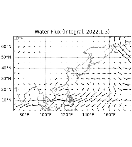
Text(0.5, 1.0, 'Water Flux (Integral, 2022.1.3)')
Total running time of the script: (0 minutes 5.731 seconds)