Curved Quiver Plot

Here is an example of how to draw a curved quiver

import easyclimate as ecl
import xarray as xr
import cartopy.crs as ccrs
import matplotlib.pyplot as plt

Import the required sample wind farm data

udata = ecl.open_tutorial_dataset("uwnd_2022_day5")["uwnd"].sortby("lat")
vdata = ecl.open_tutorial_dataset("vwnd_2022_day5")["vwnd"].sortby("lat")
uvdata = xr.Dataset(data_vars = {"u": udata,"v": vdata})
uvdata

uwnd_2022_day5.nc ━━━━━━━━━━━━━━━━━━━━ 100.0% • 2.2/2.2 MB • 60.5 MB/s • 0:00:00
vwnd_2022_day5.nc ━━━━━━━━━━━━━━━━━━━━ 100.0% • 2.2/2.2 MB • 56.3 MB/s • 0:00:00

<xarray.Dataset> Size: 7MB
Dimensions:  (time: 5, lon: 144, lat: 73, level: 17)
Coordinates:
  * time     (time) datetime64[ns] 40B 2022-01-01 2022-01-02 ... 2022-01-05
  * lon      (lon) float32 576B 0.0 2.5 5.0 7.5 10.0 ... 350.0 352.5 355.0 357.5
  * lat      (lat) float32 292B -90.0 -87.5 -85.0 -82.5 ... 82.5 85.0 87.5 90.0
  * level    (level) float32 68B 1e+03 925.0 850.0 700.0 ... 50.0 30.0 20.0 10.0
Data variables:
    u        (time, level, lat, lon) float32 4MB ...
    v        (time, level, lat, lon) float32 4MB ...

xarray.Dataset

• Dimensions:
  • time: 5
  • lon: 144
  • lat: 73
  • level: 17
• Coordinates: (4)
  • time
    (time)
    datetime64[ns]
    2022-01-01 ... 2022-01-05

    standard_name :

    time

    long_name :

    Time

    axis :

    T

    array(['2022-01-01T00:00:00.000000000', '2022-01-02T00:00:00.000000000',
           '2022-01-03T00:00:00.000000000', '2022-01-04T00:00:00.000000000',
           '2022-01-05T00:00:00.000000000'], dtype='datetime64[ns]')

  • lon
    (lon)
    float32
    0.0 2.5 5.0 ... 352.5 355.0 357.5

    standard_name :

    longitude

    long_name :

    Longitude

    units :

    degrees_east

    axis :

    X

    array([  0. ,   2.5,   5. ,   7.5,  10. ,  12.5,  15. ,  17.5,  20. ,  22.5,
            25. ,  27.5,  30. ,  32.5,  35. ,  37.5,  40. ,  42.5,  45. ,  47.5,
            50. ,  52.5,  55. ,  57.5,  60. ,  62.5,  65. ,  67.5,  70. ,  72.5,
            75. ,  77.5,  80. ,  82.5,  85. ,  87.5,  90. ,  92.5,  95. ,  97.5,
           100. , 102.5, 105. , 107.5, 110. , 112.5, 115. , 117.5, 120. , 122.5,
           125. , 127.5, 130. , 132.5, 135. , 137.5, 140. , 142.5, 145. , 147.5,
           150. , 152.5, 155. , 157.5, 160. , 162.5, 165. , 167.5, 170. , 172.5,
           175. , 177.5, 180. , 182.5, 185. , 187.5, 190. , 192.5, 195. , 197.5,
           200. , 202.5, 205. , 207.5, 210. , 212.5, 215. , 217.5, 220. , 222.5,
           225. , 227.5, 230. , 232.5, 235. , 237.5, 240. , 242.5, 245. , 247.5,
           250. , 252.5, 255. , 257.5, 260. , 262.5, 265. , 267.5, 270. , 272.5,
           275. , 277.5, 280. , 282.5, 285. , 287.5, 290. , 292.5, 295. , 297.5,
           300. , 302.5, 305. , 307.5, 310. , 312.5, 315. , 317.5, 320. , 322.5,
           325. , 327.5, 330. , 332.5, 335. , 337.5, 340. , 342.5, 345. , 347.5,
           350. , 352.5, 355. , 357.5], dtype=float32)

  • lat
    (lat)
    float32
    -90.0 -87.5 -85.0 ... 87.5 90.0

    standard_name :

    latitude

    long_name :

    Latitude

    units :

    degrees_north

    axis :

    Y

    array([-90. , -87.5, -85. , -82.5, -80. , -77.5, -75. , -72.5, -70. , -67.5,
           -65. , -62.5, -60. , -57.5, -55. , -52.5, -50. , -47.5, -45. , -42.5,
           -40. , -37.5, -35. , -32.5, -30. , -27.5, -25. , -22.5, -20. , -17.5,
           -15. , -12.5, -10. ,  -7.5,  -5. ,  -2.5,   0. ,   2.5,   5. ,   7.5,
            10. ,  12.5,  15. ,  17.5,  20. ,  22.5,  25. ,  27.5,  30. ,  32.5,
            35. ,  37.5,  40. ,  42.5,  45. ,  47.5,  50. ,  52.5,  55. ,  57.5,
            60. ,  62.5,  65. ,  67.5,  70. ,  72.5,  75. ,  77.5,  80. ,  82.5,
            85. ,  87.5,  90. ], dtype=float32)

  • level
    (level)
    float32
    1e+03 925.0 850.0 ... 20.0 10.0

    standard_name :

    air_pressure

    long_name :

    Level

    units :

    millibar

    positive :

    down

    axis :

    Z

    actual_range :

    [1000. 10.]

    GRIB_id :

    100

    GRIB_name :

    hPa

    array([1000.,  925.,  850.,  700.,  600.,  500.,  400.,  300.,  250.,  200.,
            150.,  100.,   70.,   50.,   30.,   20.,   10.], dtype=float32)

• Data variables: (2)
  • u
    (time, level, lat, lon)
    float32
    ...

    long_name :

    mean Daily U-wind

    units :

    m/s

    precision :

    2

    GRIB_id :

    33

    GRIB_name :

    UGRD

    var_desc :

    u-wind

    level_desc :

    Pressure Levels

    statistic :

    Mean

    parent_stat :

    Individual Obs

    dataset :

    NCEP Reanalysis Daily Averages

    actual_range :

    [-83.05 116.85]

    [893520 values with dtype=float32]

  • v
    (time, level, lat, lon)
    float32
    ...

    long_name :

    mean Daily V wind

    units :

    m/s

    precision :

    2

    GRIB_id :

    34

    GRIB_name :

    VGRD

    var_desc :

    v-wind

    level_desc :

    Pressure Levels

    statistic :

    Mean

    parent_stat :

    Individual Obs

    dataset :

    NCEP Reanalysis Daily Averages

    actual_range :

    [-85.925 88.125]

    [893520 values with dtype=float32]

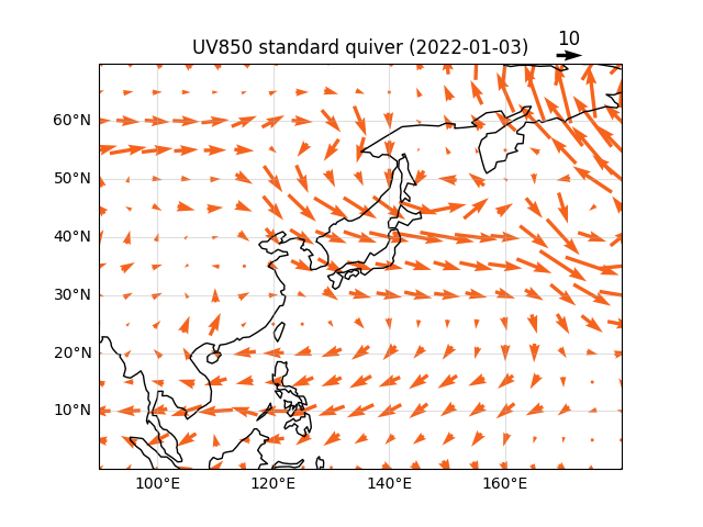
East Asia Sample

Consideration of surface wind field data for the East Asian region

lonlat_range = [90, 180, 0, 70]
gap_value = 5

drawdata_gap1 = uvdata.isel(time = 2).sel(level = 850).sel(
    lon = slice(lonlat_range[0] - gap_value, lonlat_range[1] + gap_value),
    lat = slice(lonlat_range[2] - gap_value, lonlat_range[3] + gap_value)
)

Plotting the results of a traditional quiver

fig, ax = plt.subplots(subplot_kw={"projection": ccrs.PlateCarree(central_longitude=120)})

ax.coastlines()
ax.gridlines(crs=ccrs.PlateCarree(), draw_labels=["bottom", "left"], alpha = 0.4)
ax.set_extent(lonlat_range, crs = ccrs.PlateCarree())

q = drawdata_gap1.plot.quiver(
    x = 'lon', y = 'lat', u = 'u', v = 'v',
    ax = ax,
    color = '#f6631c',  zorder = 0,
    width = 0.007,
    regrid_shape = 15,
    scale = 200,
    add_guide = False,
    transform = ccrs.PlateCarree(),
)

qk = ax.quiverkey(
    q, 0.9, 1.02,
    10, "10", labelpos = "N",
    color = "k",
    coordinates = "axes",
    fontproperties = {"size": 12},
    labelsep = 0.05,
    transform = ccrs.PlateCarree(),
)

ax.set_title("UV850 standard quiver (2022-01-03)")

Text(0.5, 1.0, 'UV850 standard quiver (2022-01-03)')

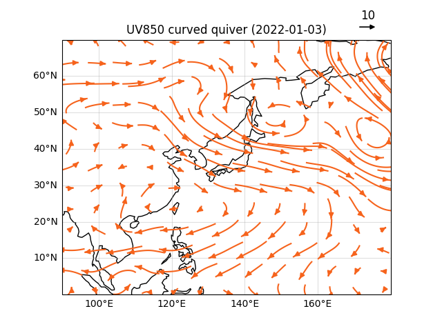
Now use a curved quiver to plot the wind field

fig, ax = plt.subplots(subplot_kw={"projection": ccrs.PlateCarree(central_longitude=120)})

ax.coastlines()
ax.gridlines(crs=ccrs.PlateCarree(), draw_labels=["bottom", "left"], alpha = 0.4)
ax.set_extent(lonlat_range, crs = ccrs.PlateCarree())

cq = ecl.plot.curved_quiver(
    drawdata_gap1,
    x = 'lon', y = 'lat', u = 'u', v = 'v',
    ax = ax,
    density = 5,
    color = '#f6631c',
    transform = ccrs.PlateCarree(),
)

ecl.plot.add_curved_quiverkey(
    cq, ax = ax,
    pos = (0.9, 1.05),
    U = 10,
    label = "10",
    color = "black",
    labelpos = "N",
    fontproperties = {"size": 12},
    ref_point = (120, 30)
)

ax.set_title("UV850 curved quiver (2022-01-03)")

Text(0.5, 1.0, 'UV850 curved quiver (2022-01-03)')

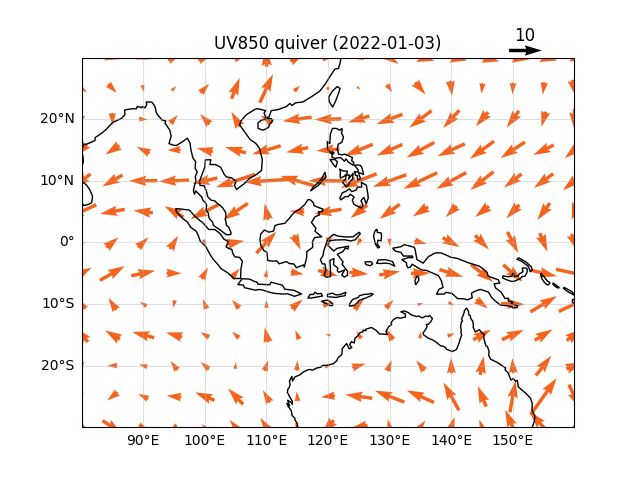
Maritime Continent Sample

Here, we will use an oceanic-continental region as an example of a wind farm in a tropical area.

gap_value = 5
lonlat_range = [80, 160, -30, 30]
drawdata_gap6 = uvdata.isel(time = 2).sel(level = 850).sel(
    lon = slice(lonlat_range[0] - gap_value, lonlat_range[1] + gap_value),
    lat = slice(lonlat_range[2] - gap_value, lonlat_range[3] + gap_value)
)

Similarly, first plot the results of the traditional Quiver wind field visualization.

fig, ax = plt.subplots(subplot_kw={"projection": ccrs.PlateCarree(central_longitude=120)})

ax.coastlines()
ax.gridlines(crs=ccrs.PlateCarree(), draw_labels=["bottom", "left"], alpha = 0.4)
ax.set_extent(lonlat_range, crs = ccrs.PlateCarree())

q = drawdata_gap6.plot.quiver(
    x = 'lon', y = 'lat', u = 'u', v = 'v',
    ax = ax,
    color = '#f6631c',  zorder = 0,
    width = 0.007,
    regrid_shape = 13,
    scale = 150,
    add_guide = False,
    transform = ccrs.PlateCarree(),
)

qk = ax.quiverkey(
    q, 0.9, 1.02,
    10, "10", labelpos = "N",
    color = "k",
    coordinates = "axes",
    fontproperties = {"size": 12},
    labelsep = 0.05,
    transform = ccrs.PlateCarree(),
)
qk.set_zorder(7)

ax.set_title("UV850 quiver (2022-01-03)")

Text(0.5, 1.0, 'UV850 quiver (2022-01-03)')

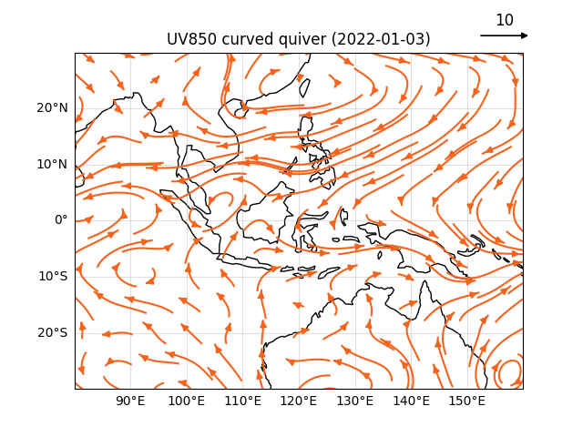
However, this is the result of drawing a curved quiver

fig, ax = plt.subplots(subplot_kw={"projection": ccrs.PlateCarree(central_longitude=120)})

ax.coastlines()
ax.gridlines(crs=ccrs.PlateCarree(), draw_labels=["bottom", "left"], alpha = 0.4)
ax.set_extent(lonlat_range, crs = ccrs.PlateCarree())

cq = ecl.plot.curved_quiver(
    drawdata_gap6,
    x = 'lon', y = 'lat', u = 'u', v = 'v',
    ax = ax,
    density = 5,
    color = '#f6631c',
    transform = ccrs.PlateCarree(),
)

ecl.plot.add_curved_quiverkey(
    cq, ax = ax,
    pos = (0.9, 1.05),
    U = 10,
    label = "10",
    color = "black",
    labelpos = "N",
    fontproperties = {"size": 12},
    ref_point = (120, 30),
)

ax.set_title("UV850 curved quiver (2022-01-03)")

Text(0.5, 1.0, 'UV850 curved quiver (2022-01-03)')

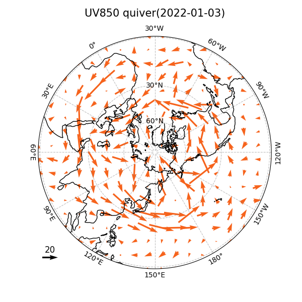
Pole Sample

Mapping the Arctic region requires additional parameter settings; here, we will first extract the data for the Arctic region.

gap_value = 5
drawdata_gap3 = uvdata.isel(time = 2).sel(level = 500).sel(
    lat = slice(0 - gap_value, None)
)
drawdata_gap3 = ecl.plot.add_lon_cyclic(drawdata_gap3, inter = 2.5)

Traditional quiver data requires an additional setting for the regrid_shape value.

fig, ax = plt.subplots(
    figsize = (6, 6),
    subplot_kw={"projection": ccrs.NorthPolarStereo(central_longitude=150)}
)
ax.coastlines()

gl, meta = ecl.plot.draw_polar_basemap(
    ax=ax,
    lon_step=30,
    lat_step=30,
    lat_range=[0, 90],
    draw_labels=True,
    lat_label_lon=-30,
    set_map_boundary_kwargs = {"south_pad": 0.9}
)

q = drawdata_gap3.plot.quiver(
    x = 'lon', y = 'lat', u = 'u', v = 'v',
    ax = ax,
    color = '#f6631c',  zorder = 0,
    width = 0.007,
    regrid_shape = 18,
    scale = 300,
    add_guide = False,
    transform = ccrs.PlateCarree(),
)

qk = ax.quiverkey(
    q, 0.05, 0.05,
    20, "20", labelpos = "N",
    color = "k",
    coordinates = "axes",
    fontproperties = {"size": 12},
    labelsep = 0.05,
    transform = ccrs.PlateCarree(),
)

ax.set_title("")
ecl.plot.set_polar_title("UV850 quiver(2022-01-03)", meta, ax, size = 15)

Text(0.5, 1.0747446830357157, 'UV850 quiver(2022-01-03)')

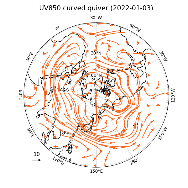
However, in a curved quiver, you need to set not only the regrid_shape but also the magnitude (ref_magnitude) and length (ref_length) of the reference vector to better plot the wind field.

fig, ax = plt.subplots(
    figsize = (6, 6),
    subplot_kw={"projection": ccrs.NorthPolarStereo(central_longitude=150)}
)
ax.coastlines()

gl, meta = ecl.plot.draw_polar_basemap(
    ax=ax,
    lon_step=30,
    lat_step=30,
    lat_range=[0, 90],
    draw_labels=True,
    lat_label_lon=-30,
    set_map_boundary_kwargs = {"south_pad": 0.9}
)

cq = ecl.plot.curved_quiver(
    drawdata_gap3,
    x = 'lon', y = 'lat', u = 'u', v = 'v',
    ax = ax,
    density = 20,
    color = '#f6631c',
    regrid_shape = 11,
    ref_magnitude = 20,
    ref_length = 0.3,
    transform = ccrs.PlateCarree(),
)

ecl.plot.add_curved_quiverkey(
    cq, ax = ax,
    pos = (0.05, 0.05),
    U = 10,
    label = "10",
    color = "black",
    labelpos = "N",
    fontproperties = {"size": 12},
    ref_point = (120, 30),
)

ax.set_title("")
ecl.plot.set_polar_title("UV850 curved quiver (2022-01-03)", meta, ax, size = 15)

Text(0.5, 1.0747446830357157, 'UV850 curved quiver (2022-01-03)')

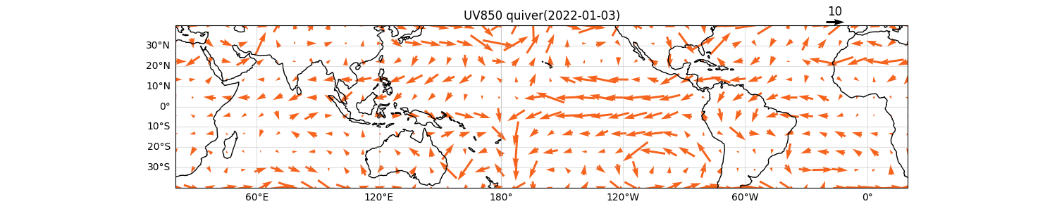
Tropics Sample

The following example covers the entire tropical region. For cases where the area is too large, additional parameters must be configured; one cannot simply rely on the default results.

gap_value = 5

lonlat_range = [0, 360, -40, 40]
drawdata_gap4 = uvdata.isel(time = 2).sel(level = 850).sel(
    lon = slice(lonlat_range[0] - gap_value, lonlat_range[1] + gap_value),
    lat = slice(lonlat_range[2] - gap_value, lonlat_range[3] + gap_value)
)
drawdata_gap4 = ecl.plot.add_lon_cyclic(drawdata_gap4, inter = 2.5)

Let’s start by looking at the rendering results for quiver.

fig, ax = plt.subplots(figsize = (15, 3) ,subplot_kw={"projection": ccrs.PlateCarree(central_longitude=200)})

ax.coastlines()
ax.gridlines(crs=ccrs.PlateCarree(), draw_labels=["bottom", "left"], alpha = 0.4)
ax.set_extent(lonlat_range, crs = ccrs.PlateCarree())

q = drawdata_gap4.plot.quiver(
    x = 'lon', y = 'lat', u = 'u', v = 'v',
    ax = ax,
    color = '#f6631c', zorder = 0,
    regrid_shape = 10,
    scale = 400,
    add_guide = False,
    transform = ccrs.PlateCarree(),
)

qk = ax.quiverkey(
    q, 0.9, 1.02,
    10, "10", labelpos = "N",
    color = "k",
    coordinates = "axes",
    fontproperties = {"size": 12},
    labelsep = 0.05,
    transform = ccrs.PlateCarree(),
)

ax.set_title("UV850 quiver(2022-01-03)")

Text(0.5, 1.0, 'UV850 quiver(2022-01-03)')

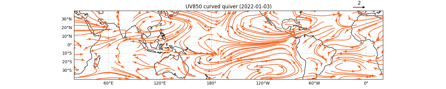
But here is the rendering result for the curved quiver.

fig, ax = plt.subplots(figsize = (15, 3),subplot_kw={"projection": ccrs.PlateCarree(central_longitude=200)})

ax.coastlines()
ax.gridlines(crs=ccrs.PlateCarree(), draw_labels=["bottom", "left"], alpha = 0.4)
ax.set_extent(lonlat_range, crs = ccrs.PlateCarree())

cq = ecl.plot.curved_quiver(
    drawdata_gap4,
    x = 'lon', y = 'lat', u = 'u', v = 'v',
    ax = ax,
    ref_magnitude = 15,
    density = 10,
    color = '#f6631c',
    regrid_shape = 15,
    transform = ccrs.PlateCarree(),
)

ecl.plot.add_curved_quiverkey(
    cq, ax = ax,
    pos = (0.9, 1.05),
    U = 2,
    label = "2",
    color = "black",
    labelpos = "N",
    fontproperties = {"size": 12},
    ref_point = (120, 30),
)

ax.set_title("UV850 curved quiver (2022-01-03)")

Text(0.5, 1.0, 'UV850 curved quiver (2022-01-03)')