Divergence¶

\[\mathrm{D} = \frac{\partial u}{\partial x} + \frac{\partial v}{\partial y} - \frac{v}{R} \tan \varphi\]

Before proceeding with all the steps, first import some necessary libraries and packages

import easyclimate as ecl
import xarray as xr
import numpy as np
import matplotlib.pyplot as plt
import cartopy.crs as ccrs
import matplotlib.ticker as mticker

Read sample data

udata = ecl.open_tutorial_dataset("uwnd_2022_day5")["uwnd"].sortby("lat")
vdata = ecl.open_tutorial_dataset("vwnd_2022_day5")["vwnd"].sortby("lat")
uvdata = xr.Dataset(data_vars = {"u": udata,"v": vdata})
uvdata

Calculating divergence using three types of functions

easyclimate.calc_divergence: Numpy Method.
easyclimate.calc_divergence_ncl: NCL Method.
easyclimate.calc_divergence_rs: Rust Method (The calculation process is similar to that of NCL, but it is faster.).

div_raw = ecl.calc_divergence(
    uvdata.u,
    uvdata.v,
)

div_ncl = ecl.calc_divergence_ncl(
    uvdata.u,
    uvdata.v,
    cyclic_boundary_setting="nan"
)

div_rust = ecl.calc_divergence_rs(
    uvdata.u,
    uvdata.v,
    cyclic_boundary_setting="nan"
)
div_rust

Plot the results of the divergence calculation

import numpy as np
import matplotlib.pyplot as plt
import cartopy.crs as ccrs
import cartopy.feature as cfeature
import matplotlib.ticker as mticker

lonlat_range = [70, 180, 0, 70]

proj = ccrs.PlateCarree()

fig, ax = plt.subplots(
    3, 1,
    figsize=(4.5, 9),
    subplot_kw={"projection": proj},
    constrained_layout=True
)

# Unify the color scale range
vmax = 2.5e-5
levels = np.linspace(-vmax, vmax, 21)
cmap = "RdBu_r"

# The three scenes that need to be drawn
fields = [
    (div_raw.isel(time=0).sel(level=850),  "div raw"),
    (div_ncl.isel(time=0).sel(level=850),  "div ncl"),
    (div_rust.isel(time=0).sel(level=850), "div rust"),
]

pcm = None

for i, (axi, (fld, title)) in enumerate(zip(ax.flat, fields)):
    axi.set_extent(lonlat_range, crs=ccrs.PlateCarree())

    # Coastlines and Base Maps
    axi.coastlines(resolution="50m", linewidth=0.8)

    # Grid lines
    gl = axi.gridlines(
        crs=ccrs.PlateCarree(),
        draw_labels=True,
        linewidth=0.5,
        color="gray",
        alpha=0.4,
        linestyle="--"
    )
    gl.top_labels = False
    gl.right_labels = False
    gl.left_labels = True
    gl.bottom_labels = True

    # It looks cleaner if you keep the bottom labels on only the bottom row.
    if i < 2:
        gl.bottom_labels = False

    gl.xlocator = mticker.FixedLocator([80, 100, 120, 140, 160, 180])
    gl.ylocator = mticker.FixedLocator([0, 10, 20, 30, 40, 50, 60, 70])

    # Drawing
    pcm = fld.plot.contourf(
        ax=axi,
        transform=ccrs.PlateCarree(),
        levels=levels,
        cmap=cmap,
        add_colorbar=False,
        extend="both"
    )

    axi.set_title(title, fontsize=13)

# Shared colorbar
cbar = fig.colorbar(
    pcm,
    ax=ax,
    orientation="horizontal",
    shrink=0.9,
    pad=0.04,
    aspect=40
)
cbar.set_label("divergence [s$^{-1}$]")

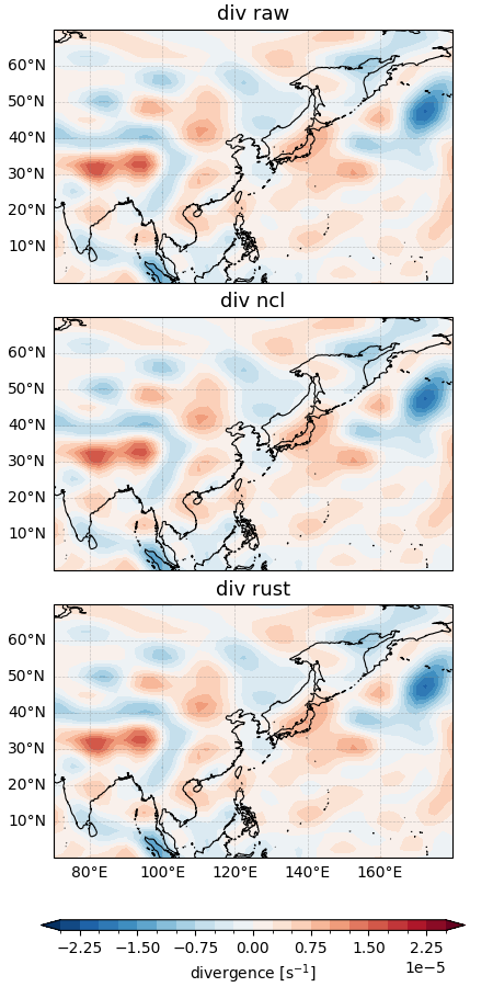
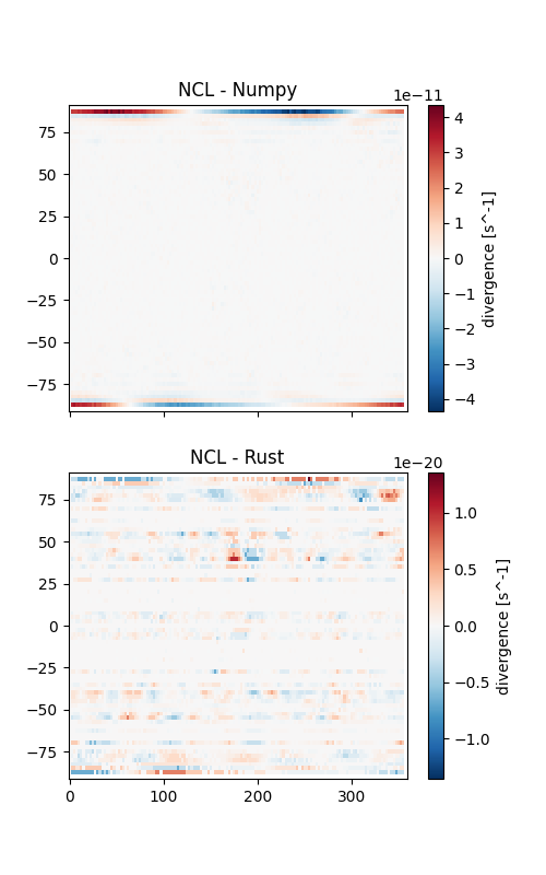
When comparing the results of different calculation methods, it is generally recommended to use the Rust-based method.

fig, ax = plt.subplots(2, 1, figsize = (5, 8), sharex=True)

(div_ncl - div_raw).isel(time = 0).sel(level = 850).plot(ax = ax[0])
ax[0].set_title("NCL - Numpy")
ax[0].set_xlabel("")
ax[0].set_ylabel("")

(div_ncl - div_rust).isel(time = 0).sel(level = 850).plot(ax = ax[1])
ax[1].set_title("NCL - Rust")
ax[1].set_xlabel("")
ax[1].set_ylabel("")

Text(18.09722222222222, 0.5, '')

Total running time of the script: (0 minutes 8.617 seconds)