Note
Go to the end to download the full example code.
zh-CN Level 1 Rivers Map
Import easyclimate-map for loading China level 1 river boundary data, matplotlib.pyplot for plotting, and cartopy.crs for map projections.
These libraries together support the retrieval and visualization of geographic data.
import easyclimate_map as eclmap
import matplotlib.pyplot as plt
import cartopy.crs as ccrs
Line
Use easyclimate_map.get_zh_CN_river1(type="line") to retrieve the line-type GeoDataFrame of China’s level 1 rivers.
This data includes river line segments and can be used to draw river courses.
zh_border_line = eclmap.get_zh_CN_nation(type = "line")
zh_river1_line = eclmap.get_zh_CN_river1(type = "line")
zh_river1_line
Use GeoPandas’ plot() method for quick visualization of the river line. This step is for initial data inspection without custom projections.
zh_river1_line.plot()
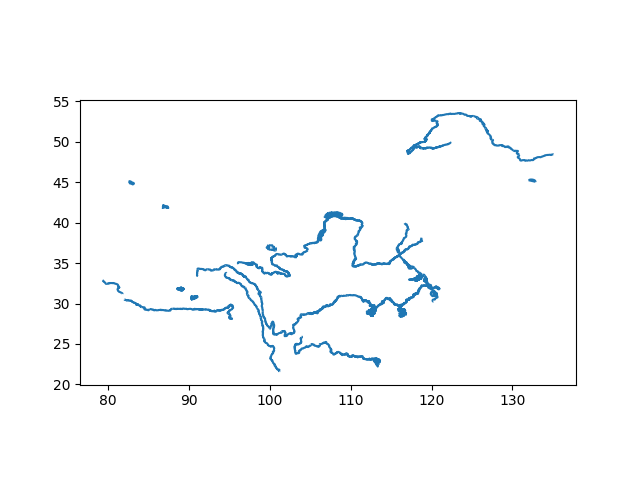
<Axes: >
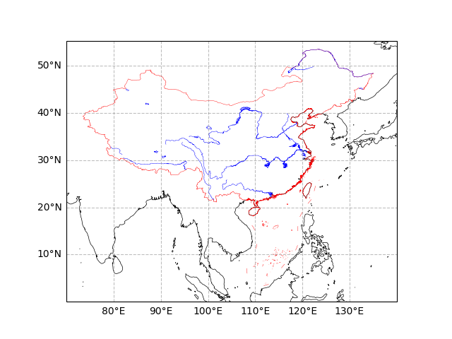
Create a subplot with PlateCarree projection (central longitude 180°), set geographic extent [70-140°E, 0-50°N]. Add gridlines, coastlines, China’s national boundary line geometries (red lines, no fill), and level 1 river line geometries (blue lines, no fill). This step demonstrates advanced map projections and geometry overlays for rivers. Parameter Details:
set_extent: Defines the map display range.
gridlines: Adds latitude/longitude grid with labels.
coastlines: Draws global coastlines (50m resolution).
add_geometries: Overlays national boundaries with red edges, line width 0.3; overlays river geometries with blue edges, line width 0.3.
fig, ax = plt.subplots(subplot_kw={"projection": ccrs.PlateCarree(central_longitude=180)})

ax.set_extent([70, 140, 0, 50])
ax.gridlines(
    draw_labels=["left", "bottom"],
    color="grey",
    alpha=0.5, linestyle="--"
)
ax.coastlines(color="k", lw = 0.5, resolution = "50m")
ax.add_geometries(
    zh_border_line.geometry,
    crs = ccrs.PlateCarree(),
    facecolor = "none",
    edgecolor = "r",
    lw = 0.3
)
ax.add_geometries(
    zh_river1_line.geometry,
    crs = ccrs.PlateCarree(),
    facecolor = "none",
    edgecolor = "b",
    lw = 0.3
)
<cartopy.mpl.feature_artist.FeatureArtist object at 0x7f299d69fc80>
Polygon
Use easyclimate_map.get_zh_CN_river1(type="polygon") to retrieve the polygon-type GeoDataFrame of China’s level 1 rivers.
This data includes closed polygon areas for river representations and can be used for area filling (e.g., wide river sections).
zh_river1_polygon = eclmap.get_zh_CN_river1(type = "polygon")
zh_river1_polygon
Use GeoPandas’ plot() method for quick visualization of the river polygon. This step is for initial data inspection without custom projections.
zh_river1_polygon.plot()
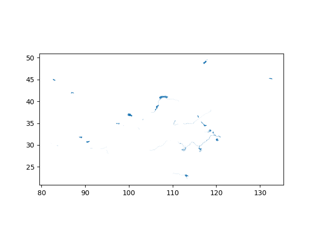
<Axes: >
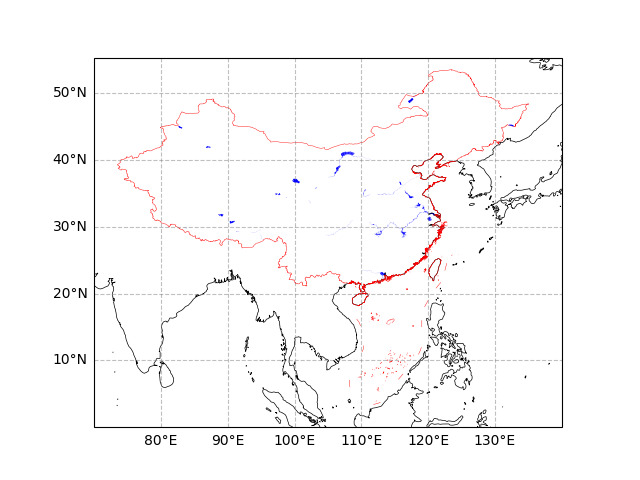
Create a subplot with PlateCarree projection (central longitude 180°), set geographic extent [70-140°E, 0-50°N]. Add gridlines, coastlines, China’s national boundary line geometries (red lines, no fill), and level 1 river polygon geometries (blue fill, no edges). This step demonstrates area fill effects for rivers, suitable for highlighting water bodies or hydrological maps. Parameter Details:
Similar to above step, but with facecolor=”b” for area fill and edgecolor=”none” for no borders on rivers.
Applicable for overlaying other data layers, such as flow directions or precipitation distributions.
fig, ax = plt.subplots(subplot_kw={"projection": ccrs.PlateCarree(central_longitude=180)})

ax.set_extent([70, 140, 0, 50])
ax.gridlines(
    draw_labels=["left", "bottom"],
    color="grey",
    alpha=0.5, linestyle="--"
)
ax.coastlines(color="k", lw = 0.5, resolution = "50m")
ax.add_geometries(
    zh_border_line.geometry,
    crs = ccrs.PlateCarree(),
    facecolor = "none",
    edgecolor = "r",
    lw = 0.3
)
ax.add_geometries(
    zh_river1_polygon.geometry,
    crs = ccrs.PlateCarree(),
    facecolor = "b",
    edgecolor = "none",
    lw = 0.3
)
<cartopy.mpl.feature_artist.FeatureArtist object at 0x7f299d43bcb0>
Total running time of the script: (0 minutes 5.696 seconds)