zh-CN First-Level Administration Centers

Import easyclimate-map for loading China first-level administration centers, matplotlib.pyplot for plotting, and cartopy.crs for map projections. These libraries together support the retrieval and visualization of geographic data.

import easyclimate_map as eclmap
import matplotlib.pyplot as plt
import cartopy.crs as ccrs
<easyclimate-map notice>: Maps are provided as-is. Users assume all risk. No
liability. No political or territorial claims.

Points

Use easyclimate_map.get_zh_CN_1st_administration() to retrieve the point-type GeoDataFrame of China’s first-level administration centers. This data includes provincial-level government seats and can be used to mark capital locations.

zh_provinces_line = eclmap.get_zh_CN_provinces(type = "line")
zh_admin1_points = eclmap.get_zh_CN_1st_administration()
zh_admin1_points
AREA PERIMETER RES1_4M_ RES1_4M_ID GBCODE NAME ADCODE93 ADCODE99 ADCLASS PINYIN geometry
0 0.0 0.0 1 61 31010 北京 110100 110100 1 Beijing POINT (116.38094 39.92361)
1 0.0 0.0 2 70 31020 天津 120100 120100 2 Tianjin POINT (117.2035 39.13112)
2 0.0 0.0 3 121 31020 石家庄 130101 130101 2 Shijiazhuang POINT (114.48978 38.04513)
3 0.0 0.0 4 220 31020 太原 140101 140101 2 Taiyuan POINT (112.56935 37.87111)
4 0.0 0.0 5 322 31020 呼和浩特 150101 150101 2 Huhehaote POINT (111.6633 40.82094)
5 0.0 0.0 6 412 31020 沈阳 210101 210101 2 Shenyang POINT (123.41168 41.79662)
6 0.0 0.0 7 465 31020 长春 220101 220101 2 Changchun POINT (125.31543 43.89256)
7 0.0 0.0 8 508 31020 哈尔滨 230101 230101 2 Haerbin POINT (126.64334 45.74149)
8 0.0 0.0 9 584 31020 上海 310100 310100 2 Shanghai POINT (121.46927 31.23818)
9 0.0 0.0 10 594 31020 南京 320101 320101 2 Nanjing POINT (118.77278 32.04762)
10 0.0 0.0 11 668 31020 杭州 330101 330101 2 Hangzhou POINT (120.15925 30.266)
11 0.0 0.0 12 741 31020 合肥 340101 340101 2 Hefei POINT (117.2757 31.86325)
12 0.0 0.0 13 823 31020 福州 350101 350101 2 Fuzhou POINT (119.29781 26.07859)
13 0.0 0.0 14 898 31020 南昌 360101 360101 2 Nanchang POINT (115.89992 28.67599)
14 0.0 0.0 15 981 31020 济南 370101 370101 2 Jinan POINT (117.0056 36.66707)
15 0.0 0.0 16 1084 31020 郑州 410101 410101 2 Zhengzhou POINT (113.65005 34.75703)
16 0.0 0.0 17 1207 31020 武汉 420101 420101 2 Wuhan POINT (114.29194 30.56751)
17 0.0 0.0 18 1344 31020 长沙 430101 430101 2 Changsha POINT (112.98127 28.20082)
18 0.0 0.0 19 1403 31020 广州 440101 440101 2 Guangzhou POINT (113.26143 23.11891)
19 0.0 0.0 20 1509 31020 南宁 450101 450101 2 Nanning POINT (108.31177 22.80654)
20 0.0 0.0 21 1580 31020 海口 460100 460100 2 Haikou POINT (110.34651 20.03179)
21 0.0 0.0 22 1620 31020 成都 510101 510101 2 Chengdu POINT (104.08176 30.66106)
22 0.0 0.0 23 1622 31030 重庆 510201 500100 2 Chongqing POINT (106.51034 29.55818)
23 0.0 0.0 24 1838 31020 贵阳 520101 520101 2 Guiyang POINT (106.71137 26.57687)
24 0.0 0.0 25 1852 31020 昆明 530101 530101 2 Kunming POINT (102.70457 25.04384)
25 0.0 0.0 26 1972 31020 拉萨 540101 540101 2 Lhasa POINT (91.13205 29.65759)
26 0.0 0.0 27 2041 31020 西安 610101 610101 2 Xi'an POINT (108.94903 34.26168)
27 0.0 0.0 28 2134 31020 兰州 620101 620101 2 Lanzhou POINT (103.75005 36.06804)
28 0.0 0.0 29 2213 31020 西宁 630100 630100 2 Xining POINT (101.78745 36.60945)
29 0.0 0.0 30 2253 31020 银川 640101 640101 2 Yinchuan POINT (106.27194 38.46801)
30 0.0 0.0 31 2274 31020 乌鲁木齐 650101 650101 2 Wulumuqi POINT (87.60612 43.79094)
31 0.0 0.0 32 2358 31020 台北 710001 710001 2 Taipei Shih POINT (121.51428 25.04913)
32 0.0 0.0 33 1384 31030 澳门 820000 820000 9 Macao POINT (113.55006 22.2008)
33 0.0 0.0 34 2377 31030 香港 810000 810000 9 Hong Kong POINT (114.1544 22.28069)


Use GeoPandas’ plot() method for quick visualization of the point locations. This step is for initial data inspection without custom projections.

zh_admin1_points.plot()
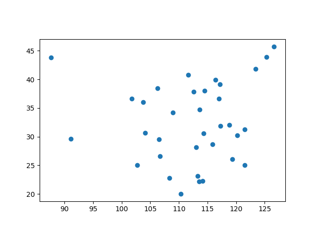
plot zh CN 1st administration
<Axes: >

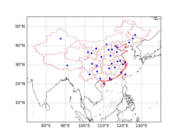
Create a subplot with PlateCarree projection (central longitude 180°), set geographic extent [70-140°E, 0-50°N]. Add gridlines, coastlines, China’s national boundary line geometries (red lines, no fill), and administration center points (blue markers). This step demonstrates point overlays for administrative centers on top of national boundaries. Parameter Details:

  • set_extent: Defines the map display range.

  • gridlines: Adds latitude/longitude grid with labels.

  • coastlines: Draws global coastlines (50m resolution).

  • add_geometries: Overlays national boundaries with red edges, line width 0.3.

  • scatter: Plots administration centers with blue markers.

fig, ax = plt.subplots(subplot_kw={"projection": ccrs.PlateCarree(central_longitude=180)})

ax.set_extent([70, 140, 0, 50])
ax.gridlines(
    draw_labels=["left", "bottom"],
    color="grey",
    alpha=0.5, linestyle="--"
)
ax.coastlines(color="k", lw = 0.5, resolution = "50m")
ax.add_geometries(
    zh_provinces_line.geometry,
    crs = ccrs.PlateCarree(),
    facecolor = "none",
    edgecolor = "r",
    lw = 0.3
)
ax.scatter(
    zh_admin1_points.geometry.x,
    zh_admin1_points.geometry.y,
    s = 12,
    color = "b",
    transform = ccrs.PlateCarree()
)
plot zh CN 1st administration
<matplotlib.collections.PathCollection object at 0x7f299d69e1b0>

Total running time of the script: (0 minutes 5.122 seconds)