zh-CN Second-Level Administration Centers

Import easyclimate-map for loading China second-level administration centers, matplotlib.pyplot for plotting, and cartopy.crs for map projections. These libraries together support the retrieval and visualization of geographic data.

import easyclimate_map as eclmap
import matplotlib.pyplot as plt
import cartopy.crs as ccrs

<easyclimate-map notice>: Maps are provided as-is. Users assume all risk. No
liability. No political or territorial claims.

Points

Use easyclimate_map.get_zh_CN_2nd_administration() to retrieve the point-type GeoDataFrame of China’s second-level administration centers. This data includes prefecture-level government seats and can be used to mark city centers.

zh_provinces_line = eclmap.get_zh_CN_provinces(type = "line")
zh_admin2_points = eclmap.get_zh_CN_2nd_administration()
zh_admin2_points

	AREA	PERIMETER	RES2_4M_	RES2_4M_ID	GBCODE	NAME	ADCODE93	ADCODE99	ADCLASS	PINYIN	geometry
0	0.0	0.0	1	1	31030	景德镇	360201	360201	3	Jingdezhen	POINT (117.11794 29.19517)
1	0.0	0.0	2	4	31030	白银	620401	620401	3	Baiyin	POINT (104.18378 36.53942)
2	0.0	0.0	3	61	31010	北京	110100	110100	1	Beijing	POINT (116.38094 39.92361)
3	0.0	0.0	4	70	31020	天津	120100	120100	2	Tianjin	POINT (117.2035 39.13112)
4	0.0	0.0	5	78	31030	唐山	130201	130201	3	Tangshan	POINT (118.20173 39.62534)
...	...	...	...	...	...	...	...	...	...	...	...
326	0.0	0.0	327	2028	31040	噶尔	542523	542523	3	Ga'er	POINT (80.09656 32.50534)
327	0.0	0.0	328	1887	31040	泽当镇	542200	542200	3	Zeetang Zhen	POINT (91.78056 29.24241)
328	0.0	0.0	329	2228	31040	八一镇	542600	542600	3	Bayi Zhen	POINT (94.35915 29.67354)
329	0.0	0.0	330	1384	31030	澳门	820000	820000	9	Macao	POINT (113.55006 22.2008)
330	0.0	0.0	331	2377	31030	香港	810000	810000	9	Hong Kong	POINT (114.1544 22.28069)

331 rows × 11 columns

Use GeoPandas’ plot() method for quick visualization of the point locations. This step is for initial data inspection without custom projections.

zh_admin2_points.plot()

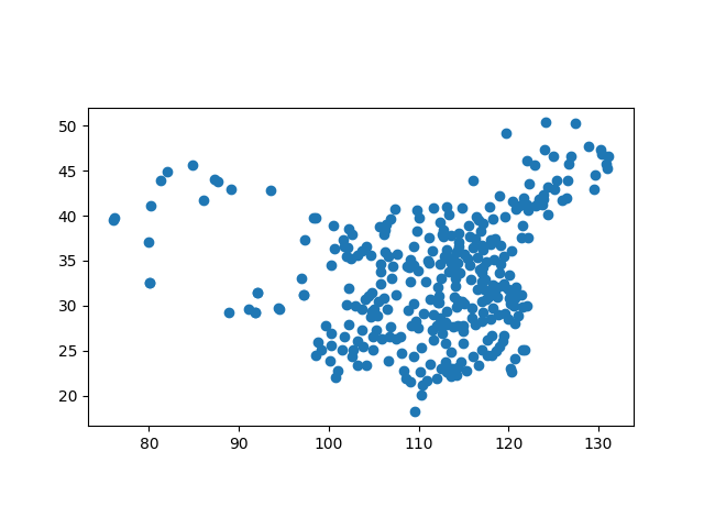
<Axes: >

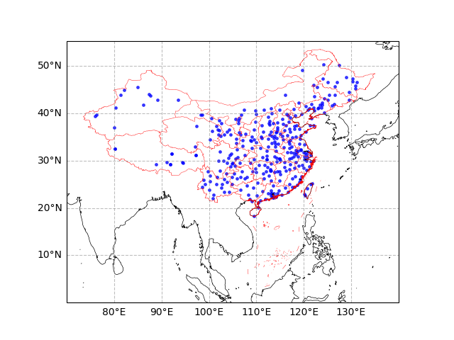
Create a subplot with PlateCarree projection (central longitude 180°), set geographic extent [70-140°E, 0-50°N]. Add gridlines, coastlines, China’s national boundary line geometries (red lines, no fill), and administration center points (blue markers). This step demonstrates dense point overlays for prefecture-level centers on top of national boundaries. Parameter Details:

• set_extent: Defines the map display range.

• gridlines: Adds latitude/longitude grid with labels.

• coastlines: Draws global coastlines (50m resolution).

• add_geometries: Overlays national boundaries with red edges, line width 0.3.

• scatter: Plots administration centers with blue markers (smaller size due to higher density).

fig, ax = plt.subplots(subplot_kw={"projection": ccrs.PlateCarree(central_longitude=180)})

ax.set_extent([70, 140, 0, 50])
ax.gridlines(
    draw_labels=["left", "bottom"],
    color="grey",
    alpha=0.5, linestyle="--"
)
ax.coastlines(color="k", lw = 0.5, resolution = "50m")
ax.add_geometries(
    zh_provinces_line.geometry,
    crs = ccrs.PlateCarree(),
    facecolor = "none",
    edgecolor = "r",
    lw = 0.3
)
ax.scatter(
    zh_admin2_points.geometry.x,
    zh_admin2_points.geometry.y,
    s = 6,
    color = "b",
    alpha = 0.7,
    transform = ccrs.PlateCarree()
)

<matplotlib.collections.PathCollection object at 0x7fb4a22d9f70>