Note
Go to the end to download the full example code.
Interpolation and Regriding#
Before proceeding with all the steps, first import some necessary libraries and packages
import easyclimate as ecl
import xarray as xr
import matplotlib.pyplot as plt
import cartopy.crs as ccrs
import numpy as np
Interpolation from points to grid (European region only)#
Open sample surface pressure data for the European region
         lat      lon     qff
0    43.8569   4.4064  1016.2
1    56.3265  -3.7273   995.1
2    55.7350  24.4170  1015.5
3    60.3000  -4.2000   997.8
4    57.8500  45.7667  1020.5
..       ...      ...     ...
867  38.8766  22.4360  1011.8
868  68.8493  28.2991  1018.2
869  39.0633  26.5983  1010.9
870  49.4464   2.1272  1009.8
871  61.3667  30.8833  1021.2

[872 rows x 3 columns]
easyclimate.interp.interp_spatial_barnes enables interpolation from site data to grid point data.
See also
Zürcher, B. K.: Fast approximate Barnes interpolation: illustrated by Python-Numba implementation fast-barnes-py v1.0, Geosci. Model Dev., 16, 1697–1711, https://doi.org/10.5194/gmd-16-1697-2023, 2023.
Plotting interpolated grid point data and corresponding station locations
fig, ax = plt.subplots(subplot_kw={"projection": ccrs.PlateCarree(central_longitude=0)})

ax.gridlines(draw_labels=["bottom", "left"], color="grey", alpha=0.5, linestyle="--")
ax.coastlines(edgecolor="black", linewidths=0.5)
ax.set_extent([-30, 15, 32, 75])

# Draw interpolation results
meshdata.plot.contourf(
    ax=ax,
    transform=ccrs.PlateCarree(),
    cbar_kwargs={"location": "bottom"},
    cmap="RdBu_r",
    levels=21,
)

# Draw observation stations
ax.scatter(data["lon"], data["lat"], s=1, c="r", transform=ccrs.PlateCarree())
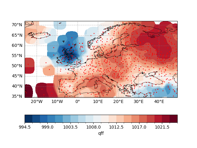
<matplotlib.collections.PathCollection object at 0x7fe72eabeb90>
Warning
The supported geographical domain and projection (as in the paper) is currently fixed to the European latitudes and Lambert conformal projection and cannot be freely chosen.
Regriding#
Reading example raw grid data
Define the target grid (only for latitude/longitude and regular grids)
target_grid = xr.DataArray(
    dims=("lat", "lon"),
    coords={
        "lat": np.arange(-89, 89, 6) + 1 / 1.0,
        "lon": np.arange(-180, 180, 6) + 1 / 1.0,
    },
)
easyclimate.interp.interp_mesh2mesh performs a regridding operation.
See also
regriding_data = ecl.interp.interp_mesh2mesh(u_data, target_grid)
regriding_data
/home/runner/work/easyclimate/easyclimate/src/easyclimate/interp/mesh2mesh.py:94: UserWarning: It seems that the input data longitude range is from -180° to 180°. Currently automatically converted to it from 0° to 360°.
  warnings.warn(
Plotting differences before and after interpolation
fig, ax = plt.subplots(1, 2, figsize=(12, 5))

u_data.sel(level=500).isel(time=0).plot(ax=ax[0])
ax[0].set_title("Before", size=20)

regriding_data.sel(level=500).isel(time=0).plot(ax=ax[1])
ax[1].set_title("After", size=20)
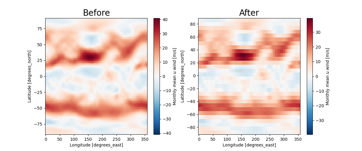
Text(0.5, 1.0, 'After')
Interpolation from model layers to altitude layers#
Suppose the following data are available
uwnd_data = xr.DataArray(
    np.array([  -15.080393 , -10.749071 ,  -4.7920494,  -2.3813725,  -1.4152431,
                -0.6465206,  -7.8181705, -14.718096 , -14.65539  , -14.948015 ,
                -13.705519 , -11.443476 ,  -8.865583 ,  -7.9528713,  -8.329103 ,
                -7.2445316,  -6.7150173,  -5.5189686,  -4.139448 ,  -3.2731838,
                -2.2931194,  -1.0041752,  -1.8983078,  -2.3674374,  -2.8203106,
                -3.2940865,  -3.526329 ,  -3.8654022,  -4.164995 ,  -4.2834396,
                -4.2950516,  -4.3438225,  -4.3716908,  -4.7688255,  -4.6155453,
                -4.5528393,  -4.4831676,  -4.385626 ,  -4.2950516,  -4.0953217]),
    dims=("model_level",),
    coords={
        "model_level": np.array([   36,  44,  51,  56,  60,  63,  67,  70,  73,  75,  78,  81,  83,
                                    85,  88,  90,  92,  94,  96,  98, 100, 102, 104, 105, 107, 109,
                                    111, 113, 115, 117, 119, 122, 124, 126, 129, 131, 133, 135, 136,
                                    137])
    },
)

p_data = xr.DataArray(
    np.array([  2081.4756,   3917.6995,   6162.6455,   8171.3506,  10112.652 ,
                11811.783 ,  14447.391 ,  16734.607 ,  19317.787 ,  21218.21  ,
                24357.875 ,  27871.277 ,  30436.492 ,  33191.027 ,  37698.96  ,
                40969.438 ,  44463.73  ,  48191.92  ,  52151.29  ,  56291.098 ,
                60525.63  ,  64770.367 ,  68943.69  ,  70979.66  ,  74908.17  ,
                78599.67  ,  82012.95  ,  85122.69  ,  87918.29  ,  90401.77  ,
                92584.94  ,  95338.72  ,  96862.08  ,  98165.305 ,  99763.38  ,
                100626.21  , 101352.69  , 101962.28  , 102228.875 , 102483.055 ]),
    dims=("model_level",),
    coords={
        "model_level": np.array([   36,  44,  51,  56,  60,  63,  67,  70,  73,  75,  78,  81,  83,
                                    85,  88,  90,  92,  94,  96,  98, 100, 102, 104, 105, 107, 109,
                                    111, 113, 115, 117, 119, 122, 124, 126, 129, 131, 133, 135, 136,
                                    137])
    },
)
Now we interpolate the data located on the mode plane to the isobaric plane. Note that the units of the given isobaric surface are consistent with pressure_data.
Simply calibrate the interpolation effect.
fig, ax = plt.subplots()
ax.plot(p_data, uwnd_data, label="Original")
ax.plot(result.plev, result.data, "o", label="Interpolated")
ax.invert_xaxis()
ax.set_xlabel("Pressure [Pa]")
ax.set_ylabel("Zonal Wind [m/s]")
plt.legend()
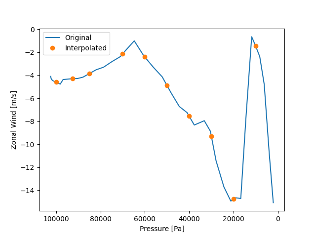
<matplotlib.legend.Legend object at 0x7fe72eeda740>
Interpolation from pressure layers to altitude layers#
Suppose the following data are available
z_data = xr.DataArray(
    np.array([  214.19354,   841.6774 ,  1516.871  ,  3055.7097 ,  4260.5806 ,
                5651.4194 ,  7288.032  ,  9288.193  , 10501.097  , 11946.71   ,
                13762.322  , 16233.451  , 18370.902  , 20415.227  , 23619.033  ,
                26214.322  , 30731.807  ]),
    dims=("level"),
    coords={
        "level": np.array([ 1000.,  925.,  850.,  700.,  600.,  500.,  400.,  300.,  250.,
                            200.,  150.,  100.,   70.,   50.,   30.,   20.,   10.])
    },
)
uwnd_data = xr.DataArray(
    np.array([  -2.3200073, -3.5700073, -2.5800018,  8.080002 , 14.059998 ,
                22.119995 , 33.819992 , 49.339996 , 57.86     , 64.009995 ,
                62.940002 , 49.809998 , 31.160004 , 16.59999  , 10.300003 ,
                10.459991 ,  9.880005 ]),
    dims=("level"),
    coords={
        "level": np.array([ 1000.,  925.,  850.,  700.,  600.,  500.,  400.,  300.,  250.,
                            200.,  150.,  100.,   70.,   50.,   30.,   20.,   10.])
    },
)
Then we need to interpolate the zonal wind data (located on the isobaric surface) to the altitude layers.
target_heights = np.linspace(0, 10000, 101)

result = ecl.interp.interp1d_vertical_pressure2altitude(
    z_data=z_data,
    variable_data=uwnd_data,
    target_heights=target_heights,
    vertical_input_dim="level",
    vertical_output_dim="altitude",
)
result
Now we can check the interpolation results.
plt.plot(z_data[:9], uwnd_data[:9], "o", label="Original")
plt.plot(result.altitude, result.data, label="Interpolated")
plt.xlabel("Altitude [m]")
plt.ylabel("Zonal Wind [m/s]")
plt.legend()
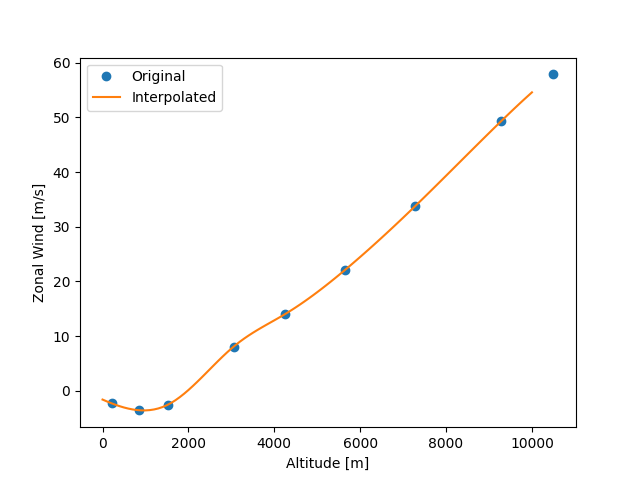
<matplotlib.legend.Legend object at 0x7fe72ea0b2e0>
Total running time of the script: (0 minutes 12.360 seconds)